Milestone 1 - Meshing the sphere

In numerical methods, we often partition the domain in smaller subdomains using what is called a mesh. The subdomains are often called grid cells, or mesh cells, or grid boxes. We will then approximate the solution to the partial differential equation that describes our model within each of those little grid cells.

The easiest way to partition a sphere is to use grid cells with uniform radius, latitude/colatitude and longitude spacings:

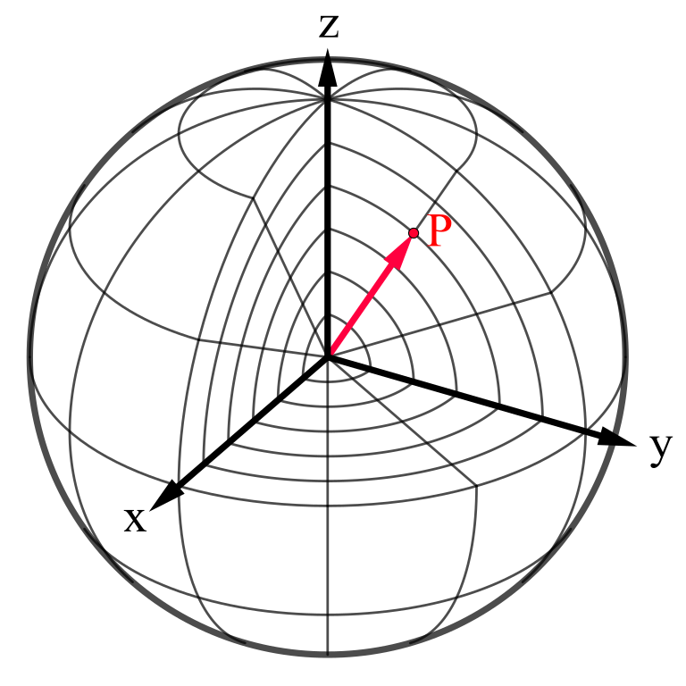
Spherical coordinate system. Source: Wikipedia (User: SharkD), CC-BY-SA 4.0.

We can observe from the figure that the grid cells get smaller the closer they are to the poles. So a regular grid in (co-)latitude and longitude space gives an irregular grid on the sphere surface. In fact, we can note that the determinant can get equal to zero for $\tilde \theta \in \{ 0, \pi\}$ . From linear algebra, we know that matrices with determinant equal to zero are not regular, i.e., they cannot be inverted. Transformations where the Jacobian matrix gets irregular are singular at this specific locations. The locations $\tilde \theta=0$ (North) and $\tilde \theta=\pi$ (South) correspond to the poles. Therefore, the transformation is singular at the poles, which shows that, regarding mappings, the poles are special locations and are somewhat problematic when trying to mesh the surface.

Because of the issues discussed above, there are many alternative ways of constructing meshes for sphere:

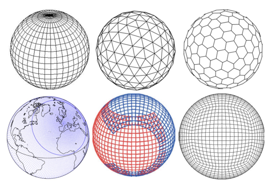
Source: Example of horizontal grid types used by atmospheric models. Weather forecasting models, Sylvie Malardel, Encyclopedia of the Environment, CC-BY-NC-SA 4.0.

For instance, the famous ICON (Icosahedral Nonhydrostatic) model from the German weather service (DWD: Deutscher Wetterdienst) uses triangle surface grids:

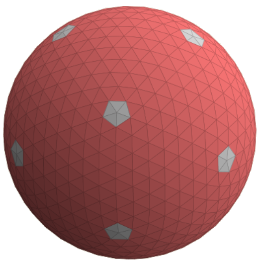
Source: Conway dcccD. Wikipedia (User:Tomruen), CC-BY-SA-4.0.

Although we have identified some issues with grids that are regular in latitude/colatitude and longitude, we have decided to use this type of grid in our model. Despite its limitations, it is the simplest grid to construct and work with. To address the singularities at the poles, we will develop and implement a special fix.

The grid that we use in this course is illustrated below:

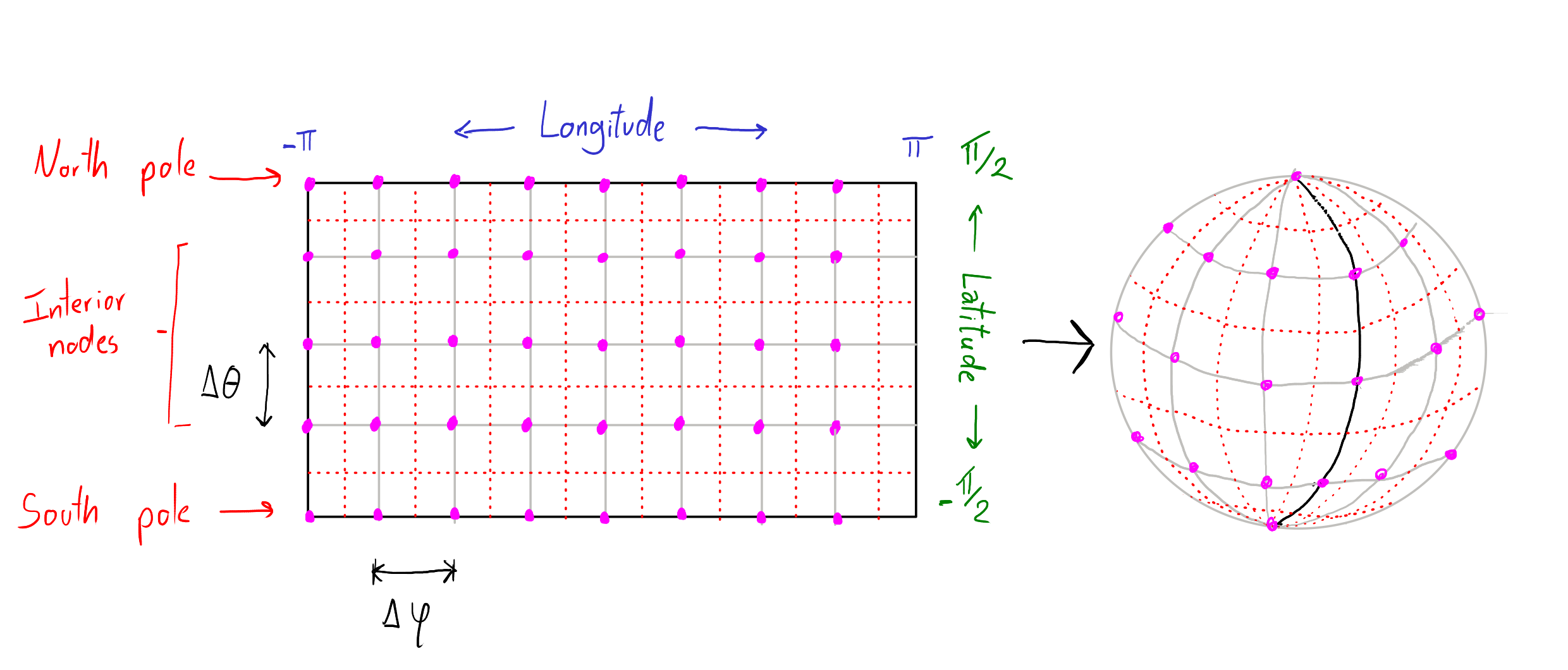
In the illustration, the boundaries of our domain are marked in blue, the grid lines of the mesh are marked in gray and the grid points of the mesh (the positions where we will store our numerical solution) are marked as purple circles.

Since our domain is periodic in the longitude direction, we do not need to store the last column of grid points ( $\varphi = \pi$ ), as their position on the surface of the sphere is the same as for the first column ( $\varphi = -\pi$ ).

Note that all the points in the first row ( $\theta = \pi/2$ ) correspond to the same position (north pole), and all the points in the last row ( $\theta = -\pi/2$ ) too (south pole). Nevertheless, we will keep these duplicated grid points in our model to simplify the storage (we can use a matrix format to store the values).

We define the number of grid points as

\begin{aligned} \texttt{n\_longitude} \in \mathbb{N} \\ \texttt{n\_latitude} \in \mathbb{N} \end{aligned}

to get the size of the grid cells as

\begin{aligned} \Delta \varphi &= \frac{2\pi}{\texttt{n\_longitude}} \\ \Delta \theta &= \Delta \tilde \theta = \frac{\pi}{\texttt{n\_latitude} -1}. \end{aligned}

To simplify the derivation of our numerical climate model, we will use uniform grids, i.e., $\Delta \varphi = \Delta \theta$ , so we require:

\texttt{n\_longitude} = 2(\texttt{n\_latitude} - 1).

The longitude grid node locations are defined from west to east

\begin{aligned} \varphi_i &= -\pi + (i-1) \Delta \varphi, & i&=1, 2, \ldots, \texttt{n\_longitude}, \end{aligned}

the latitude grid node locations are defined from north to south

\begin{aligned} \theta_j &= \frac{\pi}{2} - (j-1) \Delta \theta, & j&= 1, 2, \ldots, \texttt{n\_latitude}, \end{aligned}

and equivalently the colatitude grid node locations are

\begin{aligned} \tilde \theta_j &= (j-1) \Delta \tilde \theta, & j&= 1, 2, \ldots, \texttt{n\_latitude}. \end{aligned}

To illustrate the results of the model, we could directly plot in computational space (lat/long grid). However, it is more pleasing to the eyes and more common to plot the results in physical space (or an approximation to that). There are many options available in the literature to get from lat/long to other coordinates. In this course we use the so-called Robinson projection, which is an interesting one as this transform has no mathematical properties (it does not keep distances, angles, or areas) but was designed by Robinson by hand to look pleasing to his eyes(!).

While Robinson provided a translation table for values (lat/long), there are closed form approximations available. The form we consider was presented by

Beineke, D. (1991). Untersuchung zur Robinson-Abbildung und Vorschlag einer analytischen Abbildungsvorschrift. Kartographische Nachrichten, 41(3), 85-94.

The approximation that Beineke proposes is a simple-to-evaluate algebraic formula. Given the computational coordinates, he defines the new coordinates of the curvilinear grid as

\begin{aligned} \hat{x}_{ij} &= (d + e \theta_j^2 + f \theta_j^4 + g \theta_j^6) \varphi_i \\ x &= \frac{180}{\pi} \frac{\hat{x}_{ij}}{\max_{i,j} (\hat{x}_{ij})} \\ \hat{y}_{ij} &= a \theta_j + b \texttt{sign} (\theta_j) |\theta_j|^c \\ y &= 90 \frac{\hat{y}}{\max_{i,j} (\hat{x}_{ij})} \end{aligned}

with the parameters

\begin{aligned} a =& 0.96047, & b =& -0.00857, & c =& 6.41, \\ d =& 2.6666, & e =& -0.367, & f =& -0.150 \\ g =& 0.0379. \end{aligned}

Applying the simplified Robinson projection to the computational grid gives a curvilinear mesh a shown in the figure:

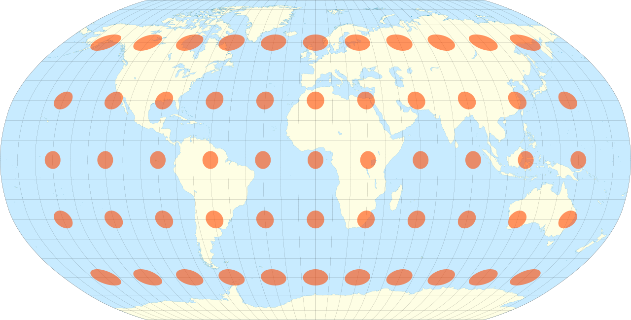
Map of the world in a Robinson projection with Tissot's Indicatrix of deformation. Source: Wikipedia (Eric Gaba - User:Sting), CC BY-SA 4.0.

As can be seen in the figure, the geographic map can be used to display the land-sea-ice-show mask of Earth, which is the topic of the first assignment, milestone 1.

Created by Gregor Gassner and Andrés Rueda-Ramírez with contributions by Simone Chiocchetti, Daniel Bach, Sophia Horak, Philipp Baasch, Benjamin Bolm, Erik Faulhaber, and Luca Sommer. Last modified: April 02, 2026. Website built with Franklin.jl and the Julia programming language.