Milestone 1 - Project Results

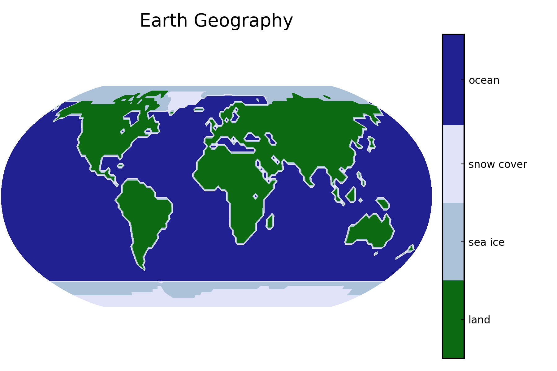
Expected Result

This is an example for the expected result:

Files Download

The Julia and Python implementations of milestone 1 can be downloaded here:

• Julia solution

• Python solution

Bonus - 3D plot

3D plot generated by Chong-Son Dröge, Fabian Höck, and Luca Levent Sommer.

Scripts for Milestone 1

You can also check out our Julia and Python implementations of milestone 1 in this site.

Julia implementation of milestone 1

using DelimitedFiles
using Plots
pythonplot()

# Creates an nlatitude x nlongitude = 65 x 128 array with integer digits decoding the geography.
function read_geography(filepath)
    return readdlm(filepath)
end

function robinson_projection(nlatitude, nlongitude)
    function x_fun(lon, lat)
        return lon / pi * (0.0379 * lat^6 - 0.15 * lat^4 - 0.367 * lat^2 + 2.666)
    end

    function y_fun(_, lat)
        return 0.96047 * lat - 0.00857 * sign(lat) * abs(lat)^6.41
    end

    # Longitude goes from -pi to pi (not included), latitude from pi/2 to -pi/2.
    # Remove endpoint of longitude to avoid overlap.
    x_lon = LinRange(-pi, pi, nlongitude + 1)[1:(end - 1)]

    # Latitude goes backwards because our plot starts at the bottom,
    # but the matrix is read from the top.
    y_lat = LinRange(pi / 2, -pi / 2, nlatitude)

    x = [x_fun(lon, lat) for lat in y_lat, lon in x_lon]
    y = [y_fun(lon, lat) for lat in y_lat, lon in x_lon]

    return x, y
end

function plot_geo(geo_dat)
    nlatitude, nlongitude = size(geo_dat)
    x, y = robinson_projection(nlatitude, nlongitude)

    # Unfortunately, this is a bit buggy. When passing a `cgrad` with `categorical=true`,
    # one would expect to only get the colors of this discrete `cgrad`, but for some reason,
    # that is not the case.
    # Instead, we got the colors that we want by experimenting with the levels.
    # We tried to make the range for ocean only slightly larger than the others to avoid
    # a weird looking colorbar.
    p = contourf(x, y, geo_dat,
                 levels=[0.5, 1.7, 2.9, 4.1, 5.5],
                 clims=(1, 5),
                 aspect_ratio=1,
                 title="Earth Geography",
                 c=cgrad([:darkgreen, :lightsteelblue, :lavender, :navy]),
                 colorbar_ticks=([1.1, 2.3, 3.5, 4.8],
                                 ["land", "sea ice", "snow cover", "ocean"]),
                 axis=([], false),
                 dpi=300)

    return p
end

# Run code
function milestone1()
    geo_dat = read_geography(joinpath(@__DIR__, "input", "The_World128x65.dat"))
    p = plot_geo(geo_dat)

    # Show the plot
    display(p)

    return p
end

Python implementation of milestone 1

import matplotlib as mpl
import matplotlib.pyplot as plt
import numpy as np


# Creates an nlatitude x nlongitude = 65 x 128 array with integer digits decoding the geography.
def read_geography(filepath):
    return np.genfromtxt(filepath, dtype=np.int8)


def robinson_projection(nlatitude, nlongitude):
    def x_fun(lon, lat):
        return lon / np.pi * (0.0379 * lat ** 6 - 0.15 * lat ** 4 - 0.367 * lat ** 2 + 2.666)

    def y_fun(_, lat):
        return 0.96047 * lat - 0.00857 * np.sign(lat) * np.abs(lat) ** 6.41

    # Longitude goes from -pi to pi (not included), latitude from -pi/2 to pi/2.
    # Latitude goes backwards because the data starts in the North, which corresponds to a latitude of pi/2.
    x_lon = np.linspace(-np.pi, np.pi, nlongitude, endpoint=False)
    y_lat = np.linspace(np.pi / 2, -np.pi / 2, nlatitude)

    x = np.array([[x_fun(lon, lat) for lon in x_lon] for lat in y_lat])
    y = np.array([[y_fun(lon, lat) for lon in x_lon] for lat in y_lat])

    return x, y


# Plot data at grid points in Robinson projection. Return the colorbar for customization.
# This will be reused in other milestones.
def plot_robinson_projection(data, title, **kwargs):
    # Get the coordinates for the Robinson projection.
    nlatitude, nlongitude = data.shape
    x, y = robinson_projection(nlatitude, nlongitude)

    # Start plotting.
    fig, ax = plt.subplots()

    # Create contour plot of geography information against x and y.
    im = ax.contourf(x, y, data, **kwargs)
    plt.title(title)
    ax.set_aspect("equal")

    # Remove axes and ticks.
    plt.xticks([])
    plt.yticks([])
    ax.spines["top"].set_visible(False)
    ax.spines["right"].set_visible(False)
    ax.spines["bottom"].set_visible(False)
    ax.spines["left"].set_visible(False)

    # Colorbar with the same height as the plot. Code copied from
    # https://stackoverflow.com/a/18195921
    # create an axes on the right side of ax. The width of cax will be 5%
    # of ax and the padding between cax and ax will be fixed at 0.05 inch.
    from mpl_toolkits.axes_grid1 import make_axes_locatable
    divider = make_axes_locatable(ax)
    cax = divider.append_axes("right", size="5%", pad=0.05)
    cbar = plt.colorbar(im, cax=cax)

    return cbar


def plot_geo(geo_dat):
    # Minimum and maximum of the values of the geography info.
    vmin = 1
    vmax = 5

    # This is a contour plot where the space between the contour levels is filled with a specific color.
    # We want our integer values to be between these contour levels, so we can, for example, choose these levels.
    # For the correct tick position, we choose the levels such that our integer values are exactly in the middle
    # between two levels.
    levels = [0.5, 1.5, 2.5, 3.5, 6.5]

    # Define colors of world map.
    cmap = mpl.colors.ListedColormap(["darkgreen", "lightsteelblue", "lavender", "navy"])

    cbar = plot_robinson_projection(geo_dat, "Earth Geography", levels=levels, cmap=cmap,
                                    vmin=vmin, vmax=vmax)
    cbar.set_ticks([1, 2, 3, 5])
    cbar.ax.set_yticklabels(["land", "sea ice", "snow cover", "ocean"])

    # Adjust size of plot to viewport to prevent clipping of the legend.
    plt.tight_layout()
    plt.show()


# Run the code.
if __name__ == "__main__":
    file = "input/The_World128x65.dat"
    geo_dat_ = read_geography(file)
    plot_geo(geo_dat_)

    nlatitude_, nlongitude_ = geo_dat_.shape
    print("nlatitude  = ", nlatitude_)
    print("nlongitude =", nlongitude_)