Milestone 2 - Albedo

We keep our momentum and focus on another parameter in our model that heavily depends on the type of the surface: the so-called albedo $\alpha$. The value $1-\alpha$ is also called co-albedo.

Albedo describes the reflectivity of the material and hence strongly depends on the details of the surface of a body. As we see in our energy balance the value of the albedo $\alpha$ plays a crucial role in the energy balance: the larger $\alpha$ the less stellar energy is in the energy balance, as part of it gets directly reflected.

Again, we are only able to use strong approximations and parametrizations of the albedo. In particular we will use a varying in space but constant in time approximation for our albedo model. It is however clear that temporal processes such as cloud cover, snow and ice change will impact the albedo in time. More precisely, the albedo, cloud cover, snow and ice etc. are closely coupled and connected via feedback mechanisms.

Assuming the main reflections to be from the type of surface in combination with a temporally averaged cloud cover, we have

where the effective albedo is

An option would be to find observational data and measurements to estimate the values of $\alpha$. We follow again closely the paper of Zhuang et al. (2017), which itself is based on a paper by Mengel et al., Seasonal snowline instability in an energy balance model, Climm Dynam, 1988.

In the parametrization of Zhuang et al. we have some base values of albedo for each surface type ($geo$) in combination with some averaged cloud cover values:

Land/soil ($geo=1$): $\alpha = 0.3$.

Sea ice ($geo=2$): $\alpha = 0.6$.

Snow cover ($geo=3$): $\alpha = 0.75$.

Lake/inland sea ($geo=4$): $\alpha = 0.3$.

Ocean ($geo=5$): $\alpha = 0.29$.

The following figures show that the albedo is dependent on the latitude $\theta$ (sine of latitude) and has almost a U-shape, with high values at the poles (ice and show) and low values at the equator. We do note, that typically, there is a discontinuity in the albedo when going from ocean/land to ice and snow due to the strong and sudden difference.

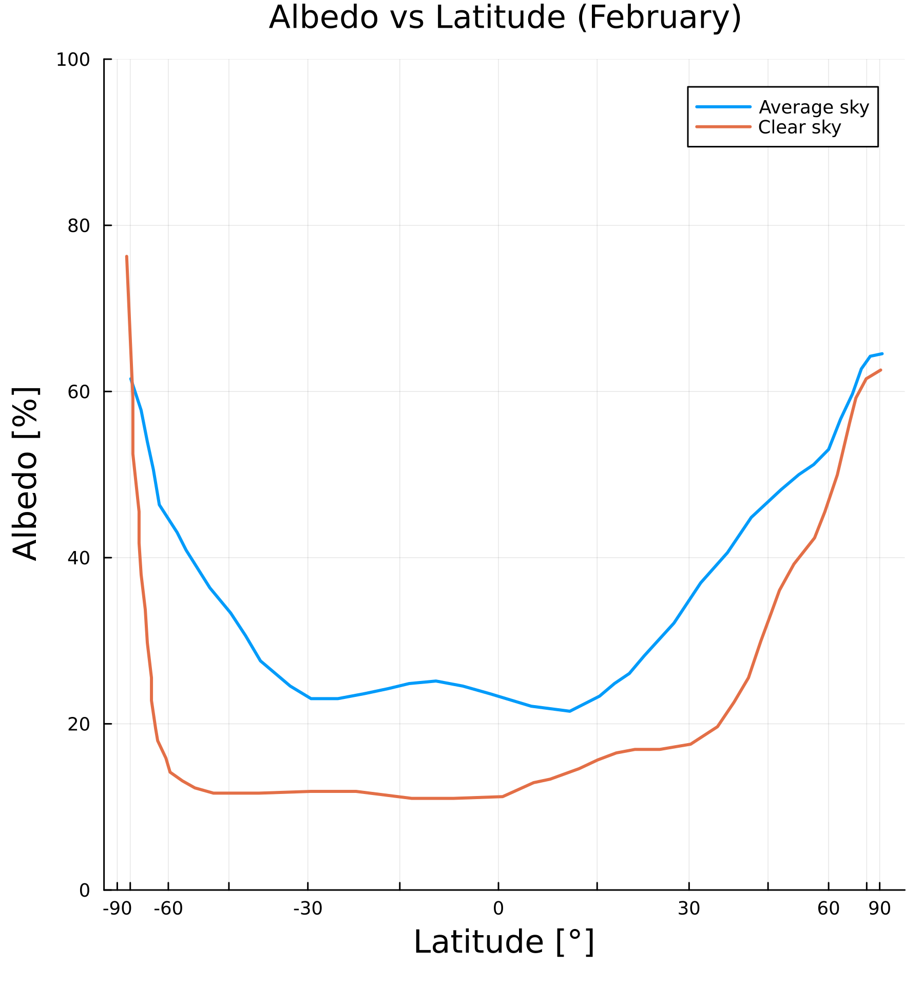
• Data from Earth Radiation Budget Experiment (ERBE) of NASA Shows the observed background and albedo for different months. Note, that the x-axis is in fact in sinusoidal scale, rather than linear.

This figure was generated with data from Graves, C. E., Lee, W. H., & North, G. R. (1993). New parameterizations and sensitivities for simple climate models. Journal of Geophysical Research: Atmospheres, 98(D3), 5025-5036.

Due to the U-shape form an approximation with a simple symmetric function as a model seems reasonable. Graves et al. (1993) do not directly use the latitude $\theta$, but the sine of the latitude, $\sin(\theta)$, and then use a quadratic polynomial as their ansatz with coefficients fitted to the data shown in the above figures. We consider a similar modification for land, ocean, and lakes ($geo=\{1,4,5\}$), which covers most Earth, except close to the poles. Consider the latitude $\theta$ given at a grid node, we can compute the value

to get the modifications

Land/soil ($geo=1$): $\alpha = 0.3 + 0.12\,p(\theta)$

Lake/inland sea ($geo=4$): $\alpha = 0.3 + 0.12\,p(\theta)$,

Ocean ($geo=5$): $\alpha = 0.29 + 0.12\,p(\theta)$,

while we keep the values for ice and snow as the constants from above. This modification makes the albedo depend on the spatial location while it keeps it independent of (constant in) time.

The following plot shows the quality of the approximation with respect to moderate latitudes.

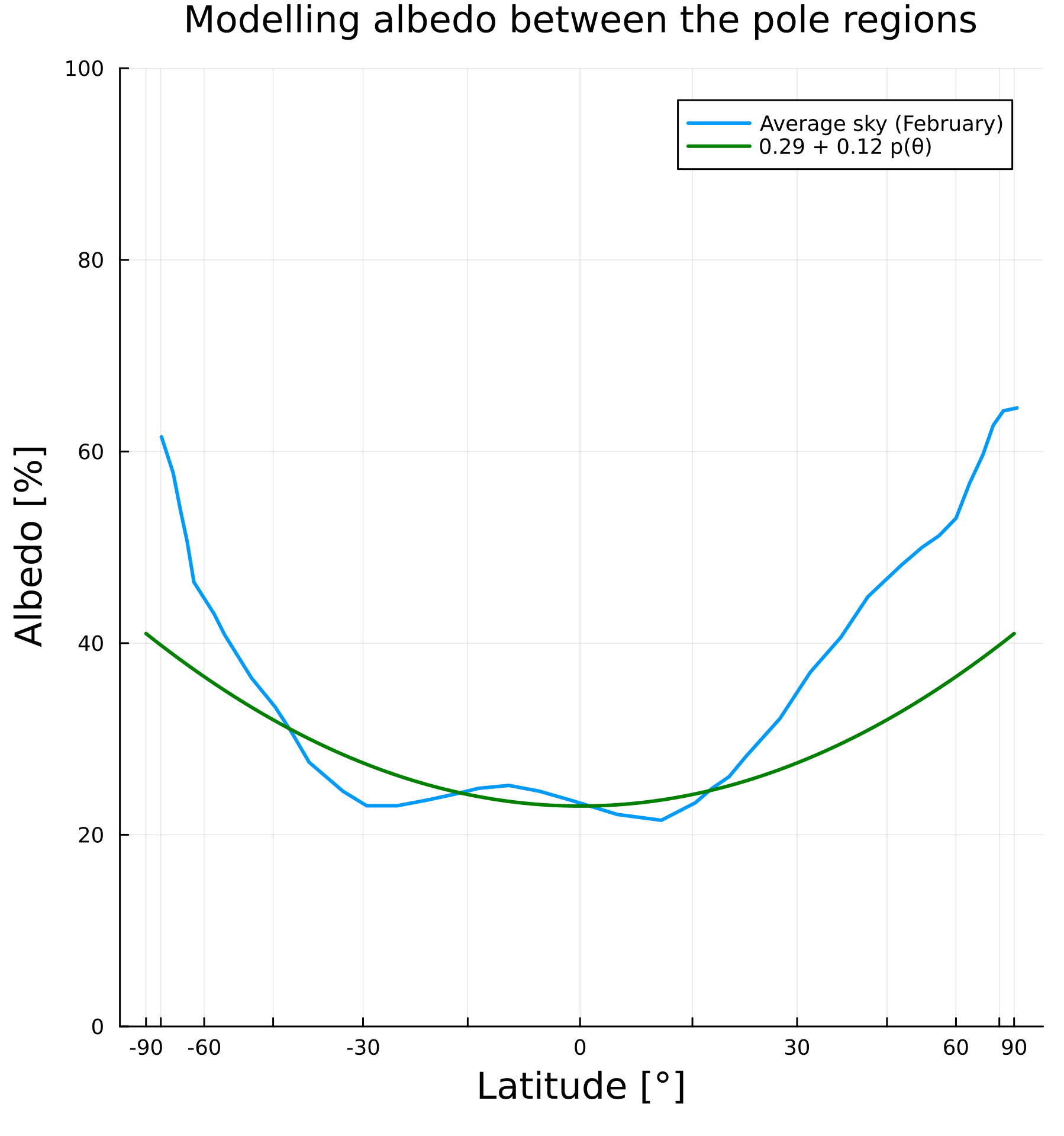
Again, this figure is showing the x-axis in sinusoidal scale and was generated with data from Graves, C. E., Lee, W. H., & North, G. R. (1993). New parameterizations and sensitivities for simple climate models. Journal of Geophysical Research: Atmospheres, 98(D3), 5025-5036.