Milestone 2 - Radiation modeling

Introduction

The energy balance of Earth is strongly impacted by radiation. The following figure shows the energy fluxes in the global Earth atmosphere system.

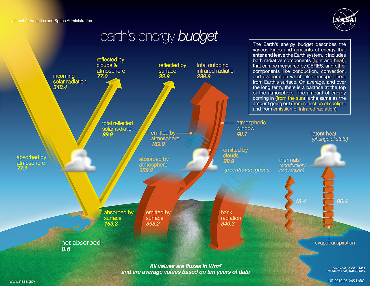
• Earth's Energy Budget. Source: NASA, Public domain, quoting Loeb et al., J. Clim 2009 & Trenberth et al, BAMS 2009.

In our EBM, we aim to include four effects:

(i) Incoming solar radiation.

(ii) Reflection of radiation by the surface and cloud cover.

(iii) Cooling because of outgoing longwave radiation.

(iv) Effect of greenhouse gases (mainly $CO_2$).

Outgoing longwave radiation

The goal in this section is to define a model/parametrization for the source term $S_{OLW}(T,x,t)$.

But first, to warm up with the topic, we consider as a toy model an idealized black-body Earth, i.e., we assume that the Earth is a black body that emits and absorbs radiation in the infrared spectrum.

The radiation energy per time that is emitted by a black body can be computed by the Stefan-Boltzmann law of physics

where $I$ is the radiation energy per time per area with units $[W/m^2]$, $T_R$ is the radiation temperature with physical units Kelvin $[K]$, $\sigma_{SB} = 0.56687\cdot 10^{-8}$ is the Stefan-Boltzmann constant with units $[W/m^2/K^4]$.

For this idealized black-body Earth, the temperature is determined when the outgoing radiation is in equilibrium/balance with the incoming stellar radiation. The amount of incoming energy can be roughly estimated as $S_0\,(1-\alpha)\,\pi\,R_E^2$, where $S_0 = 1360 [W/m^2]$ is the solar constant (the mean solar elecromagnetic radiation received on Earth), $\alpha$ is the surface albedo (the amount of the solar radiation that is reflected back to space) with the planetary average being about $\alpha=0.3$ (more details in the Albedo section), and $R_E=6.378\cdot 10^{6} [m]$ is the radius of Earth. Note that the solar constant is scaled with the effective area in which the solar radiation is applied on earth: $\pi\,R_E^2$.

Taking into account that the surface of the sphere is $4\pi R_E^2$, the amount of outgoing energy is $\sigma_{SB} T_R^4 4\,\pi\,R_E^2$, and we get our first (simplest version of an) EBM

We can relate this simple EBM (2) to the general EBM form by making the assumption of thermodynamic equilibrium (no temporal change $\partial T / \partial t= 0$), no heat diffusion ($d = 0$), and the following choice of source terms:

We can directly solve (2) to get the black-body equilibrium temperature

This model is indeed as simple as it gets and it is no surprise that the quality of the prediction of an average Earth temperature is quite off. The black-body radiation temperature of Earth would be only about $-18$ degree Celsius, hence, some major modeling improvements are necessary.

Budyko's Empirical infrared Model

Budyko (1968) suggested an empirical linear model for the outgoing longwave radiation

It is in general motivated by available observational data, shown in the next figure

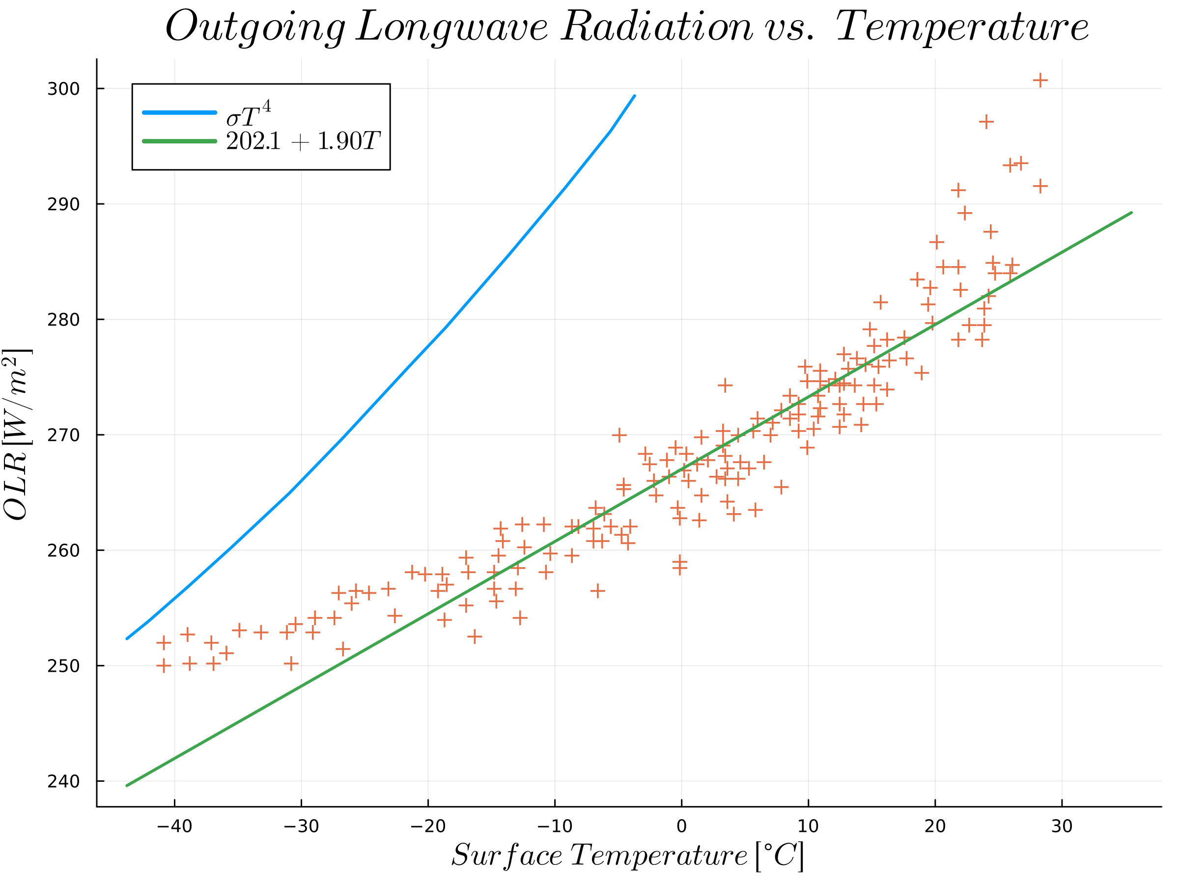
• Measured outgoing longwave radiation as a function of the surface temperature between 1975 and 1985. Generated with data from Graves, C. E., Lee, W. H., & North, G. R. (1993). New parameterizations and sensitivities for simple climate models. Journal of Geophysical Research: Atmospheres, 98(D3), 5025-5036.

The figure shows infrared radiation density plots averaged monthly, measured by satellite compared to the surface temperature at the same month and location. (a) shows the whole sky (including clouds) and (b) shows only the clear (cloudless) sky.

If we consider the temperature in units Kelvin, we can fit the observed data with the linear model by choosing good constants $A$ and $B$ to get

with $A=210.3$ as the radiative cooling in units $[W/m^2]$, and $B=2.15$ the radiative cooling feedback with units $[W/m^2/K]$. It is important to note that the choice of these parameters has a direct impact on the outgoing radiation and hence on the cooling. Several others have fitted the data differently, hence some range of choices for $A$ and $B$ is available. The values we select are from the paper by Zhuang et al. (2017).

We are now able to consider a second, but hopefully improved toy EBM. We replace the crude black-body radiation with a phenomenological approximation of the outgoing radiation (the Budyko model) to get

which can be directly solved again to get the equilibrium temperature

Effect of greenhouse gases ($CO_2$)

For the interested reader, we refer to chapter 4 of the book by Kim and North, "Energy Balance Climate Model", (2017, Wiley) and the following paper

Myhre, G., Highwood, E. J., Shine, K. P., & Stordal, F. (1998). New estimates of radiative forcing due to well mixed greenhouse gases. Geophysical research letters, 25(14), 2715-2718.

The Earth's atmosphere is composed of several gases, with the most abundant ones being nitrogen ($N_2$), oxygen ($O_2$), and argon ($Ar$). These gases do not strongly absorb infrared radiation, which is important because the Earth's surface emits infrared radiation as it cools down after being heated by the sun. $N_2$ and $O_2$ are diatomic molecules, meaning they consist of two atoms chemically bonded together. Diatomic molecules have no permanent dipole, which means they have no separation of electric charge and therefore do not strongly interact with infrared radiation. Argon, on the other hand, is a monatomic gas, meaning it consists of individual atoms rather than molecules. However, it does not absorb infrared radiation because it does not have any modes of rotation or vibration in the infrared spectrum.

Overall, the lack of strong absorption of infrared radiation by these main constituents of the atmosphere allows heat to escape from the Earth's surface and be radiated out to space, helping to regulate the planet's temperature.

$H_2O$ molecules, on the other hand, have a permanent dipole moment because the distribution of electrons in the molecule is asymmetric. As a result, $H_2O$ molecules respond strongly to passing electromagnetic waves, including those in the infrared spectrum, which leads to the absorption of infrared radiation.

Molecules such as $CO_2$, $CH_4$, and $NO_2$ do not have a permanent dipole moment because they are symmetrical in shape. However, they can still absorb infrared radiation through the phenomenon of induced dipole moments. When an infrared photon passes near one of these molecules, it can cause the electrons in the molecule to shift slightly, resulting in a temporary dipole moment. This temporary dipole moment can then interact with the passing electromagnetic wave, leading to the absorption of infrared radiation.

The ability of these molecules to absorb infrared radiation is significant because it allows them to contribute to the greenhouse effect. The greenhouse effect is the process by which certain gases in the Earth's atmosphere, including $CO_2$, $CH_4$, and $NO_2$, trap heat and warm the planet's surface. Without this natural process, the Earth's average temperature would be much lower and life as we know it would not be possible. However, when these gases are present in excess, they can cause an imbalance in the greenhouse effect, leading to climate change.

In this course, we follow the paper by Myhre et al. (1998) to define our parametrization of the greenhouse gas effect. From this paper, we first look at the effect of the amount of greenhouse gases, as plotted in the following figures:

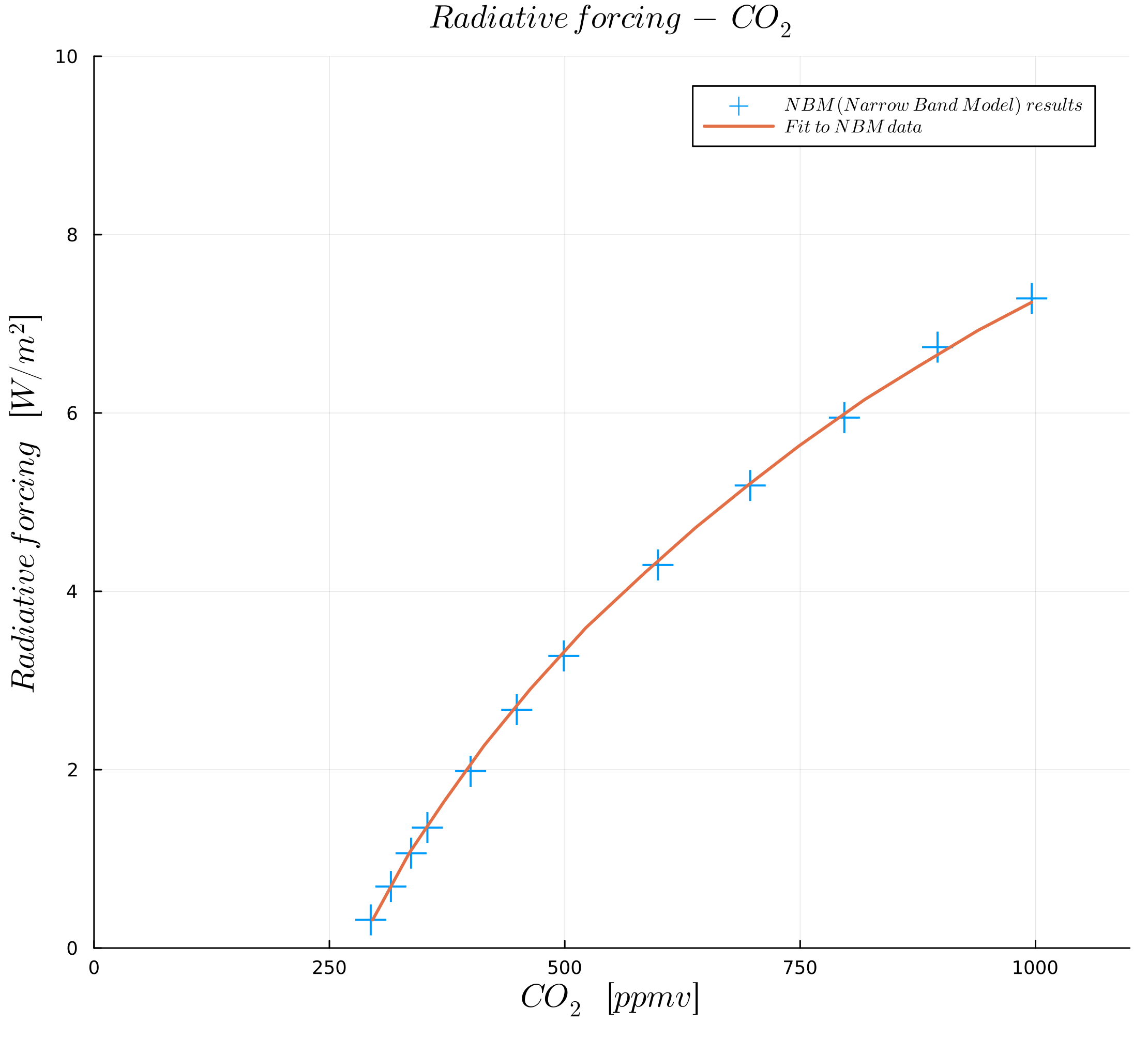
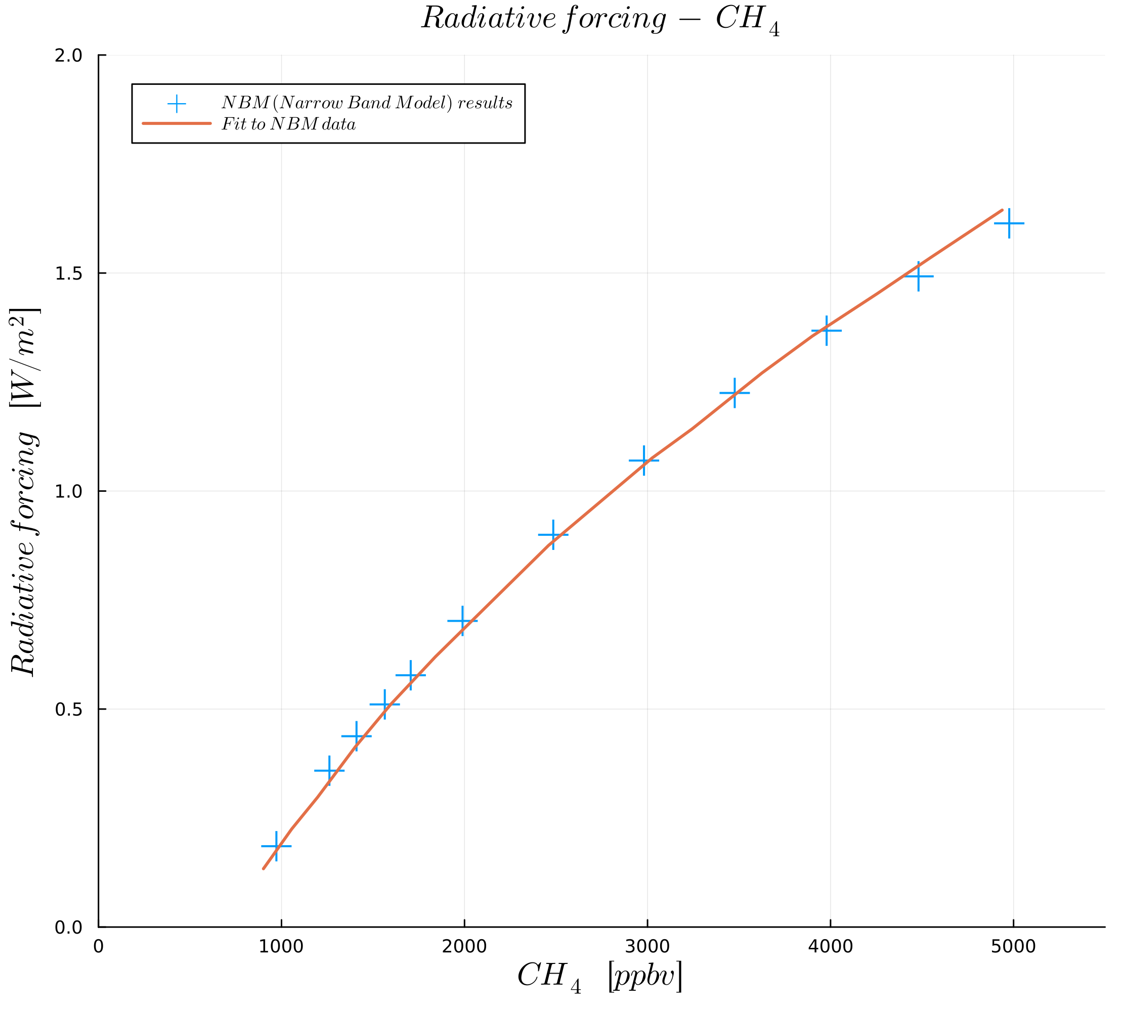
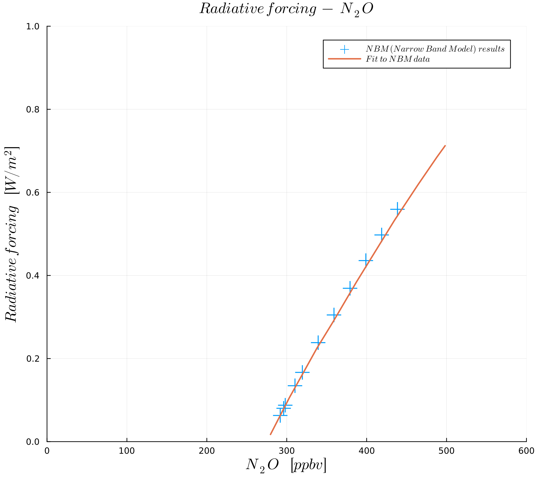
• Figures were generated with data from Myhre et al. (1998).

The figures show radiative forcing as a function of concentration in $[ppmv]$ ("parts per million by volume") for $CO_2$ and in $[ppbv]$ ("parts per billion by volume") for $CH_4$ and $N_2O$.

The following table gathers simplified expressions to compute (fit) the radiative forcing caused by different greenhouse gases using data from Myhre et al. (1998) and the function

• Table: Simplified expressions for the radiative forcing $\Delta A$ in $[W/m^2]$ with coefficients of the IPCC report (1990) and Myhre et al. (1998). In the expressions, $C$ is CO$_2$ concentration in $[ppmv]$, $M$ is CH$_4$ concentration in $[ppbv]$, $N$ is N$_2$O concentration in $[ppbv]$, and $X$ is Chlorofluorocarbons (CFCs) concentration in $[ppbv]$. The subscript $0$ denotes unperturbed (reference) concentrations. The function $f$ is given in (9). Adapted from Myhre et al. (1998).

As mentioned, we only consider the effect of $CO_2$ in our model and hence choose the approximation

where

$CO_2$ is the concentration in $[ppm]$, and $CO_2(t_0) = 315\, [ppm]$ is the reference concentration in the year $t_0 = 1950$.

In summary, we get the following parametrization of our outgoing longwave radiation source term

which we reformulate into the shorthand notation

where

and

where we further made the assumption that the unit of the temperature $T$ is $[^\circ C]$ instead of Kelvin.