Milestone 2 - Project Results

Expected Results

This is an example for the expected results:

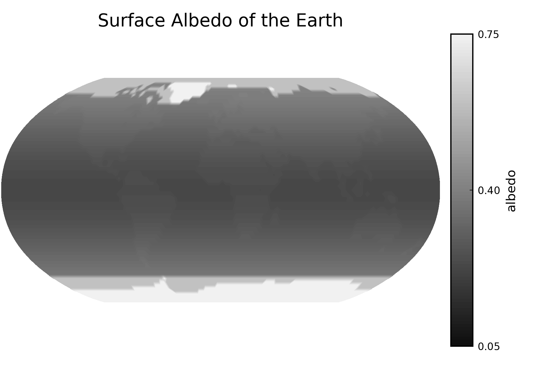
Albedo Plot

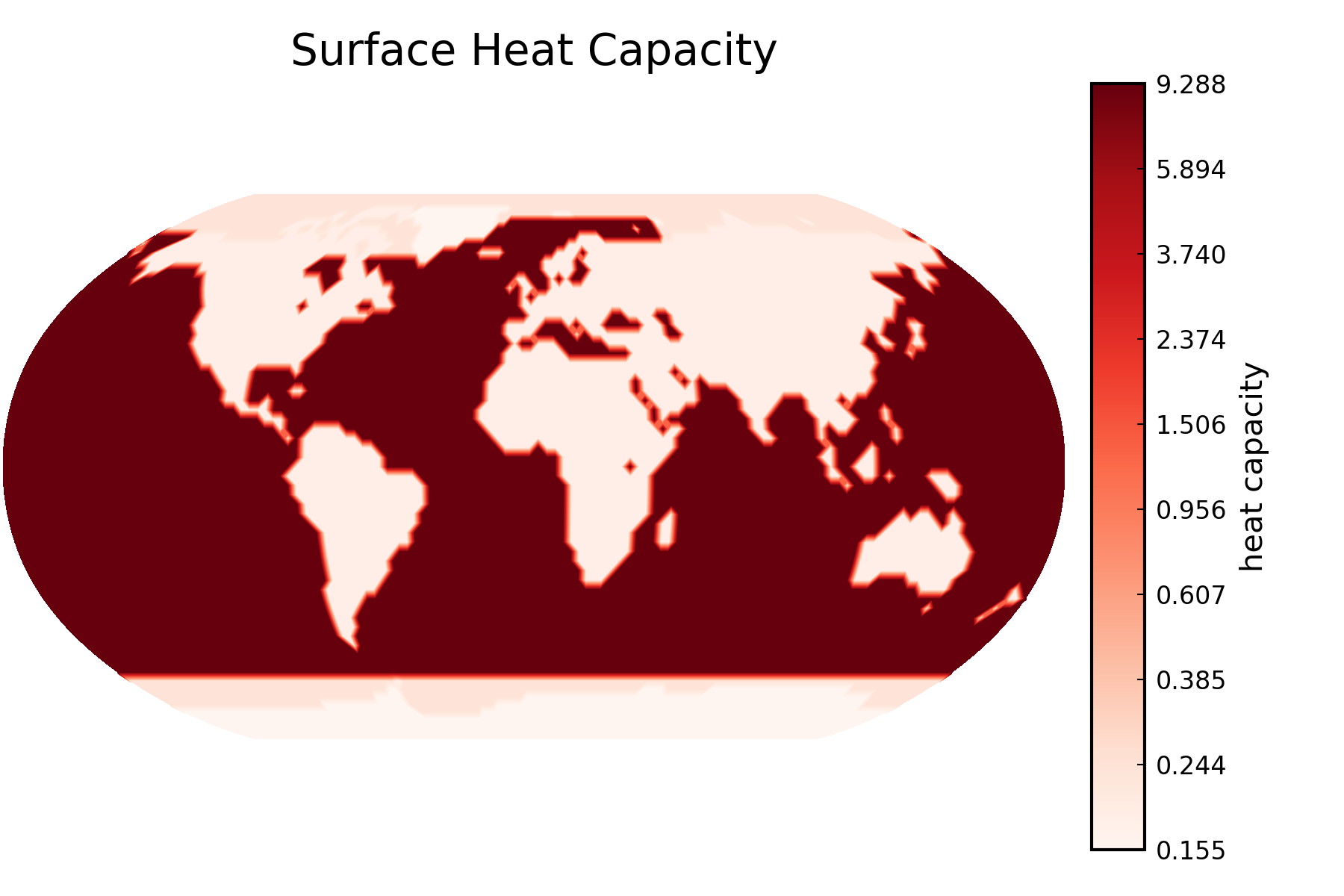
Heat Capacity Plot

Solar Forcing Animation

Files Download

The Julia and Python implementations of milestone 2 can be downloaded here:

• Julia solution

• Python solution

Bonus - 3D plots

3D plots generated by Chong-Son Dröge, Fabian Höck, and Luca Levent Sommer.

Scripts for Milestone 2

You can also check out our Julia and Python implementations of milestone 2 in this site.

Julia implementation of milestone 2

using DelimitedFiles
using Plots
using Printf
pythonplot()

include("milestone1.jl")

function calc_albedo(geo_dat)
    legendre(latitude) = 0.5 * (3 * sin(latitude)^2 - 1)

    function albedo(surface_type, latitude)
        if surface_type == 1
            return 0.3 + 0.12 * legendre(latitude)
        elseif surface_type == 2
            return 0.6
        elseif surface_type == 3
            return 0.75
        elseif surface_type == 5
            return 0.29 + 0.12 * legendre(latitude)
        else
            error("Unknown surface type $surface_type.")
        end
    end

    nlatitude, nlongitude = size(geo_dat)
    y_lat = LinRange(pi / 2, -pi / 2, nlatitude)

    # Map surface type to albedo.
    return [albedo(geo_dat[i, j], y_lat[i]) for i in 1:nlatitude, j in 1:nlongitude]
end

function plot_albedo(albedo)
    # Minimum and maximum of the values of the albedo.
    vmin = 0.05
    vmax = maximum(albedo)

    # Plot as in milestone 1
    nlatitude, nlongitude = size(albedo)
    x, y = robinson_projection(nlatitude, nlongitude)

    plot = contourf(x, y, albedo,
                    clims=(vmin, vmax),
                    levels=LinRange(vmin, vmax, 100),
                    aspect_ratio=1,
                    title="Surface Albedo of the Earth",
                    c=:grays,
                    colorbar_title="albedo",
                    colorbar_ticks=([vmin, 0.5 * (vmin + vmax), vmax]),
                    axis=([], false),
                    dpi=300)

    return plot
end

function calc_heat_capacity(geo_dat)
    sec_per_yr = 3.15576e7 # seconds per year

    c_atmos = 1.225 * 1000 * 3850
    c_ocean = 1030 * 4000 * 70
    c_seaice = 917 * 2000 * 1.5
    c_land = 1350 * 750 * 1
    c_snow = 400 * 880 * 0.5

    function heat_capacity(surface_type)
        if surface_type == 1
            capacity_surface = c_land
        elseif surface_type == 2
            capacity_surface = c_seaice
        elseif surface_type == 3
            capacity_surface = c_snow
        elseif surface_type == 5
            capacity_surface = c_ocean
        else
            error("Unknown surface type $surface_type.")
        end

        return (capacity_surface + c_atmos) / sec_per_yr
    end

    # Map surface type to heat capacity.
    nlatitude, nlongitude = size(geo_dat)
    return [heat_capacity(geo_dat[i, j]) for i in 1:nlatitude, j in 1:nlongitude]
end

function plot_heat_capacity(heat_capacity)
    # Unfortunately, Julia Plots seems to not offer the functionality to plot
    # against a logarithmic colorbar. Let's do this manually.
    heat_capacity_log = log10.(heat_capacity)

    vmin = minimum(heat_capacity_log)
    vmax = maximum(heat_capacity_log)

    # Plot as in milestone 1
    nlatitude, nlongitude = size(heat_capacity_log)
    x, y = robinson_projection(nlatitude, nlongitude)

    cbar_ticks = LinRange(vmin, vmax, 10)
    cbar_tick_values = [@sprintf("%.3f", 10^tick) for tick in cbar_ticks]

    plot = contourf(x, y, heat_capacity_log,
                    clims=(vmin, vmax),
                    levels=LinRange(vmin, vmax, 500),
                    aspect_ratio=1,
                    title="Surface Heat Capacity",
                    c=:Reds,
                    colorbar_title="heat capacity",
                    colorbar_ticks=(cbar_ticks, cbar_tick_values),
                    axis=([], false),
                    dpi=300)

    return plot
end

function read_true_longitude(filepath)
    return readdlm(filepath)
end

function insolation(latitude, true_longitude, solar_constant, eccentricity,
                    obliquity, precession_distance)
    # Determine if there is no sunset or no sunrise.
    sin_delta = sin(obliquity) * sin(true_longitude)
    cos_delta = sqrt(1 - sin_delta^2)
    tan_delta = sin_delta / cos_delta

    # Note that z can be +-infinity.
    # This is not a problem, as it is only used for the comparison with +-1.
    # We will never enter the `else` case below if z is +-infinity.
    z = -tan(latitude) * tan_delta

    if z >= 1
        # Latitude where there is no sunrise
        return 0.0
    else
        rho = ((1 - eccentricity * cos(true_longitude - precession_distance)) /
               (1 - eccentricity^2))^2

        if z <= -1
            # Latitude where there is no sunset
            return solar_constant * rho * sin(latitude) * sin_delta
        else
            h0 = acos(z)
            second_term = h0 * sin(latitude) * sin_delta +
                          cos(latitude) * cos_delta * sin(h0)
            return solar_constant * rho / pi * second_term
        end
    end
end

function calc_solar_forcing(albedo, true_longitudes, solar_constant=1371.685,
                            eccentricity=0.01674, obliquity=0.409253,
                            precession_distance=1.783037)
    function solar_forcing(theta, true_longitude, albedo_loc)
        s = insolation(theta, true_longitude, solar_constant, eccentricity,
                       obliquity, precession_distance)
        a_c = 1 - albedo_loc

        return s * a_c
    end

    # Latitude values at the grid points
    nlatitude, nlongitude = size(albedo)
    y_lat = LinRange(pi / 2, -pi / 2, nlatitude)

    return [solar_forcing(y_lat[i], true_longitude, albedo[i, j])
            for i in 1:nlatitude, j in 1:nlongitude, true_longitude in true_longitudes]
end

function plot_solar_forcing(solar_forcing, timestep)
    # Minimum and maximum of the values of the albedo.
    vmin = minimum(solar_forcing)
    vmax = maximum(solar_forcing)

    # Plot as in milestone 1
    nlatitude, nlongitude = size(solar_forcing)
    x, y = robinson_projection(nlatitude, nlongitude)

    ntimesteps = size(solar_forcing, 3)
    day = (round(Int, (timestep - 1) / ntimesteps * 365) + 80) % 365
    plot = contourf(x, y, solar_forcing[:, :, timestep],
                    clims=(vmin, vmax),
                    levels=LinRange(vmin, vmax, 200),
                    aspect_ratio=1,
                    title="Solar Forcing for Day $day",
                    c=:gist_heat,
                    colorbar_title="solar forcing",
                    axis=([], false),
                    dpi=300)

    return plot
end

# Run code
function milestone2()
    geo_dat = read_geography(joinpath(@__DIR__, "input", "The_World128x65.dat"))

    # Plot albedo
    albedo = calc_albedo(geo_dat)
    plot_albedo_ = plot_albedo(albedo)

    # Plot heat capacity
    heat_capacity = calc_heat_capacity(geo_dat)
    plot_heat_capacity_ = plot_heat_capacity(heat_capacity)

    # Compute solar forcing
    true_longitude = read_true_longitude(joinpath(@__DIR__, "input", "True_Longitude.dat"))
    solar_forcing = calc_solar_forcing(albedo, true_longitude)

    # Plot solar forcing for each time step
    anim = @animate for ts in 1:length(true_longitude)
        plot_solar_forcing(solar_forcing, ts)
    end

    gif_solar_forcing = gif(anim, joinpath(@__DIR__, "solar_forcing.gif"), fps=7)

    # Show all plots and the animation
    display(plot_albedo_)
    display(plot_heat_capacity_)
    display(gif_solar_forcing)

    return plot_albedo_, plot_heat_capacity_, gif_solar_forcing
end

Python implementation of milestone 2

import os

import imageio
import matplotlib.pyplot as plt
import numpy as np
from matplotlib.colors import LogNorm
from matplotlib.ticker import ScalarFormatter

from milestone1 import read_geography, plot_robinson_projection


def calc_albedo(geo_dat):
    def legendre(latitude):
        return 0.5 * (3 * np.sin(latitude) ** 2 - 1)

    def albedo(surface_type, latitude):
        if surface_type == 1:
            return 0.3 + 0.12 * legendre(latitude)
        elif surface_type == 2:
            return 0.6
        elif surface_type == 3:
            return 0.75
        elif surface_type == 5:
            return 0.29 + 0.12 * legendre(latitude)
        else:
            raise ValueError(f"Unknown surface type {surface_type}.")

    nlatitude, nlongitude = geo_dat.shape
    y_lat = np.linspace(np.pi / 2, -np.pi / 2, nlatitude)

    # Map surface type to albedo.
    return np.array([[albedo(geo_dat[i, j], y_lat[i])
                      for j in range(nlongitude)]
                     for i in range(nlatitude)])


def plot_albedo(albedo):
    # Minimum and maximum of the values of the albedo.
    vmin = 0.05  # np.amin(albedo)
    vmax = np.amax(albedo)

    levels = np.linspace(vmin, vmax, 100)

    # Reuse plotting function from milestone 1.
    cbar = plot_robinson_projection(albedo, "Surface Albedo of the Earth",
                                    levels=levels, cmap="gray",
                                    vmin=vmin, vmax=vmax)
    cbar.set_ticks([vmin, 0.5 * (vmin + vmax), vmax])
    cbar.set_label("albedo")

    # Adjust size of plot to viewport to prevent clipping of the legend.
    plt.tight_layout()
    plt.show()


def calc_heat_capacity(geo_dat):
    sec_per_yr = 3.15576e7  # seconds per year

    c_atmos = 1.225 * 1000 * 3850
    c_ocean = 1030 * 4000 * 70
    c_seaice = 917 * 2000 * 1.5
    c_land = 1350 * 750 * 1
    c_snow = 400 * 880 * 0.5

    def heat_capacity(surface_type):
        if surface_type == 1:
            capacity_surface = c_land
        elif surface_type == 2:
            capacity_surface = c_seaice
        elif surface_type == 3:
            capacity_surface = c_snow
        elif surface_type == 5:
            capacity_surface = c_ocean
        else:
            raise ValueError(f"Unknown surface type {surface_type}.")

        return (capacity_surface + c_atmos) / sec_per_yr

    # Map surface type to heat capacity.
    nlatitude, nlongitude = geo_dat.shape
    return np.array([[heat_capacity(geo_dat[i, j])
                      for j in range(nlongitude)]
                     for i in range(nlatitude)])


def plot_heat_capacity(heat_capacity):
    vmin = np.amin(heat_capacity)
    vmax = np.amax(heat_capacity)

    levels = np.power(10, np.linspace(np.log10(vmin), np.log10(vmax), 500))

    # Reuse plotting function from milestone 1.
    cbar = plot_robinson_projection(heat_capacity, "Surface Heat Capacity",
                                    levels=levels, cmap="Reds",
                                    vmin=vmin, vmax=vmax, norm=LogNorm())

    cbar.set_label("heat capacity")
    # `norm=LogNorm()` above sets the formatter to a LogFormatter by default
    cbar.formatter = ScalarFormatter()

    # Adjust size of plot to viewport to prevent clipping of the legend.
    plt.tight_layout()
    plt.show()


def read_true_longitude(filepath):
    return np.genfromtxt(filepath, dtype=np.float64)


def insolation(latitude, true_longitude, solar_constant, eccentricity,
               obliquity, precession_distance):
    # Determine if there is no sunset or no sunrise.
    sin_delta = np.sin(obliquity) * np.sin(true_longitude)
    cos_delta = np.sqrt(1 - sin_delta ** 2)
    tan_delta = sin_delta / cos_delta

    # Note that z can be +-infinity.
    # This is not a problem, as it is only used for the comparison with +-1.
    # We will never enter the `else` case below if z is +-infinity.
    z = -np.tan(latitude) * tan_delta

    if z >= 1:
        # Latitude where there is no sunrise
        return 0.0
    else:
        rho = ((1 - eccentricity * np.cos(true_longitude - precession_distance))
               / (1 - eccentricity ** 2)) ** 2

        if z <= -1:
            # Latitude where there is no sunset
            return solar_constant * rho * np.sin(latitude) * sin_delta
        else:
            h0 = np.arccos(z)
            second_term = h0 * np.sin(latitude) * sin_delta + np.cos(latitude) * cos_delta * np.sin(h0)
            return solar_constant * rho / np.pi * second_term


def calc_solar_forcing(albedo, true_longitudes, solar_constant=1371.685,
                       eccentricity=0.01674, obliquity=0.409253,
                       precession_distance=1.783037):
    def solar_forcing(theta, true_longitude, albedo_loc):
        s = insolation(theta, true_longitude, solar_constant, eccentricity,
                       obliquity, precession_distance)
        a_c = 1 - albedo_loc

        return s * a_c

    # Latitude values at the grid points
    nlatitude, nlongitude = albedo.shape
    y_lat = np.linspace(np.pi / 2, -np.pi / 2, nlatitude)

    return np.array([[[solar_forcing(y_lat[i], true_longitude, albedo[i, j])
                       for true_longitude in true_longitudes]
                      for j in range(nlongitude)]
                     for i in range(nlatitude)])


def plot_solar_forcing(solar_forcing, timestep, show_plot=False):
    vmin = np.amin(solar_forcing)
    vmax = np.amax(solar_forcing) * 1.05
    levels = np.linspace(vmin, vmax, 200)

    # Reuse plotting function from milestone 1.
    ntimesteps = solar_forcing.shape[2]
    day = (np.int_(timestep / ntimesteps * 365) + 80) % 365
    cbar = plot_robinson_projection(solar_forcing[:, :, timestep],
                                    f"Solar Forcing for Day {day}",
                                    levels=levels, cmap="gist_heat",
                                    vmin=vmin, vmax=vmax)
    cbar.set_label("solar forcing")

    # Adjust size of plot to viewport to prevent clipping of the legend.
    plt.tight_layout()

    filename = 'solar_forcing_{}.png'.format(timestep)
    plt.savefig(filename, dpi=300)
    if show_plot:
        plt.show()
    plt.close()

    return filename


# Run code
if __name__ == '__main__':
    geo_dat_ = read_geography("input/The_World128x65.dat")

    # Plot albedo
    albedo_ = calc_albedo(geo_dat_)
    plot_albedo(albedo_)

    # Plot heat capacity
    heat_capacity_ = calc_heat_capacity(geo_dat_)
    plot_heat_capacity(heat_capacity_)

    # Compute solar forcing
    true_longitude_ = read_true_longitude("input/True_Longitude.dat")
    solar_forcing_ = calc_solar_forcing(albedo_, true_longitude_)

    # Plot solar forcing for each time step
    filenames = []
    for ts in range(len(true_longitude_)):
        filename_ = plot_solar_forcing(solar_forcing_, ts, show_plot=False)
        filenames.append(filename_)

    # Build GIF
    frames = [imageio.v3.imread(filename_) for filename_ in filenames]
    imageio.mimsave("solar_forcing.gif", frames)

    # Remove files
    for filename_ in set(filenames):
        os.remove(filename_)