Milestone 3 - Averages

As mentioned, we need to be careful when computing spatial averages because of the spherical coordinate system. We need the averaging procedures to (i) define our simplified models, (ii) to later analyze the numerical results that we get, e.g., compute the average temperature in the southern hemisphere. We further need to define temporal averaging and apply all of this to our field data, such as, e.g., the temperature itself, the heat capacity, or the solar forcing terms.

Area average

We have to be careful about computing the area average: while we use a Cartesian computational grid in longitude and latitude, we need the average over the sphere surface.

We consider the latitude/longitude grid:

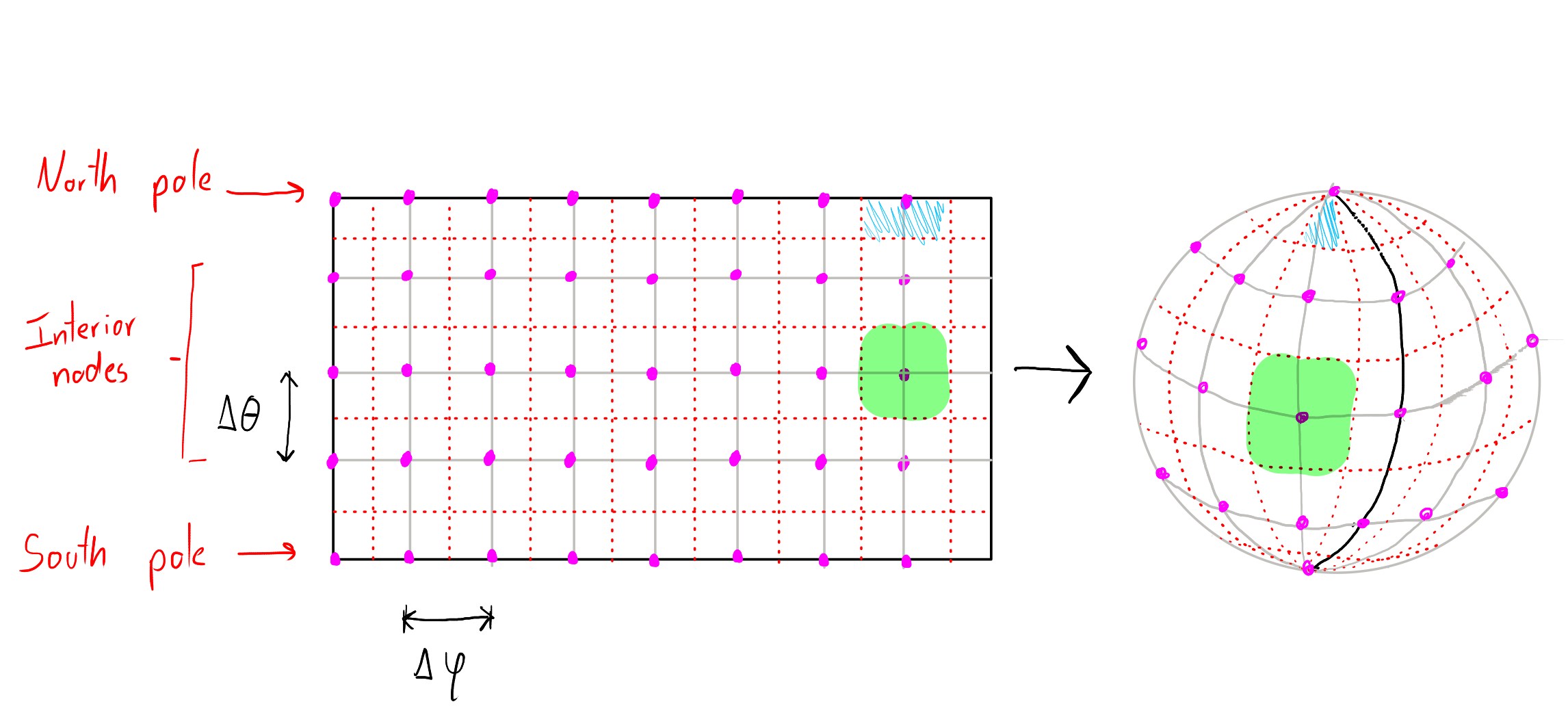
In the figure, the discretization nodes are marked in purple, the grid lines are marked in gray, and we have drawn additional auxiliary grid lines (dotted lines in red) between our computational nodes. We are going to use these auxiliary grid lines to define the surface area that corresponds to each computational node.

The area average of a field $F(x)$ that takes the value $F_{ji}$ at each node $ji$ can be in general written as

where $\omega_{ji}$ contains the normalized areas for each of the grid points of our mesh.

Observe that, even though we use a regular grid, the area that corresponds to each computational node of our grid depends only on the latitude, and not on the longitude. Therefore, our goal is to compute the corresponding approximation of the area for each latitude grid coordinate $\theta_j$.

In addition, observe that each node at the pole maps to a triangle, and not to a quadrilateral. In preparation for the discretization of the diffusion operator in spherical coordinates (Milestone 5), we already start to treat the pole regions ($j=1$ and $j=\texttt{n\_latitude}$) in a special way.

Poles (North and South)

We need to compute the area of a spherical cap at the angle $\theta = \frac{\Delta \theta}{2}$.

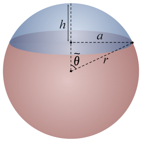
• Spherical cap diagram. Modified from Wikipedia (User:Jhmadden), CC-BY-SA 4.0.

Using standard geometrical formulae, we can derive the area of a spherical cap with radius $R_E$ as

As we will use the area calculation only to compute area averages of quantities on the surface of the sphere, we will directly normalize this value with the surface area of the Earth (sphere), i.e.

Interior nodes

For the interior nodes, we consider a spherical segment between the two angles $(\theta_j - \Delta \theta/2)$ and $(\theta_j + \Delta \theta/2)$. We can use (3) to compute the difference between two spherical caps and obtain

Implementation and data structures

To compute the area average of a vector containing values at the grid points, we will directly store the normalized area entries ($\omega_{ij}$ of equation (1)) in a vector of floats with length $\texttt{n\_latitude}$ that we will call area.

For instance, assuming $\texttt{n\_latitude} = 65$, we can declare the vector in Julia as

n_latitude = 65
n_longitude = 2 * (n_latitude - 1)
area = zeros(Float64, n_latitude)

The grid size is

Therefore, taking into account that Julia uses one-based indexing we have for the poles

delta_theta = pi / (n_latitude - 1)
area[1] = 0.5 * (1 - cos(0.5 * delta_theta))
area[n_latitude] = area[1]

Next, we store the area of the interior grid points, however, with a twist:

for j=2:n_latitude-1
    theta_j = delta_theta * (j - 1)
    area[j] = sin(0.5 * delta_theta) * sin(theta_j) / n_longitude
end
# We print the area array to check that everything is right
println(area)

To obtain:

[0.00015059065189787502, 9.407664130914078e-6, 1.8792664374922727e-5, 2.8132391444409192e-5, 3.740434511879961e-5, 4.658618844956514e-5, 5.5655801571887494e-5, 6.45913349933507e-5, 7.337126223128217e-5, 8.19744316719349e-5, 9.038011752657774e-5, 9.856806976173572e-5, 0.00010651856288329443, 0.0001142124434569431, 0.00012163117625047545, 0.00012875688888678758, 0.00013557241489999997, 0.0001420613350909772, 0.00014820801708261686, 0.0001539976529796154, 0.00015941629504198472, 0.0001644508892863796, 0.00016908930693428686, 0.00017332037363131534, 0.00017713389636719423, 0.00018052068803162764, 0.00018347258954684803, 0.00018598248952354917, 0.000188044341392846, 0.0001896531779729884, 0.00019080512343573738, 0.00019149740264357476, 0.00019172834783525225, 0.00019149740264357476, 0.0001908051234357374, 0.0001896531779729884, 0.000188044341392846, 0.00018598248952354917, 0.00018347258954684803, 0.00018052068803162764, 0.00017713389636719423, 0.00017332037363131537, 0.00016908930693428686, 0.0001644508892863796, 0.00015941629504198475, 0.0001539976529796154, 0.00014820801708261688, 0.00014206133509097718, 0.0001355724149, 0.00012875688888678763, 0.00012163117625047545, 0.00011421244345694313, 0.00010651856288329443, 9.856806976173573e-5, 9.038011752657778e-5, 8.197443167193489e-5, 7.337126223128218e-5, 6.459133499335076e-5, 5.56558015718875e-5, 4.658618844956518e-5, 3.740434511879968e-5, 2.8132391444409203e-5, 1.8792664374922768e-5, 9.40766413091407e-6, 0.00015059065189787502]

With this, we get an easy formula for the calculation of the area average of a given field F(j,i) with $j=1, \ldots, \texttt{n\_latitude}$ and $i=1, \ldots, \texttt{n\_longitude}$.

function calc_mean(field, area, n_latitude, n_longitude)
  if size(field)[1] !== n_latitude || size(field)[2] !== n_longitude
    error("field and area sizes do not match")
  end

  # Initialize mean with the values at the poles
  mean = area[1]*field[1,1] + area[end]*field[end,end]

  for j in 2:n_latitude-1
      for i in 1:n_longitude
          mean += area[j] * field[j,i]
      end 
  end

  return mean
end

We test our routine by computing the area average of the data $F(j,i)=1, \; \forall (j,i)$ to get the value of $1$.

field = ones(Float64,n_latitude,n_longitude)
println("Area : ", calc_mean(field, area, n_latitude, n_longitude))
println("Error: ", calc_mean(field, area, n_latitude, n_longitude)-1)

When we execute the code, we obtain:

Area : 1.0000000000000027
Error: 2.6645352591003757e-15

Temporal average

The temporal average is less involved and relatively straightforward. We make the assumption that the temporal behavior is periodic with perdiodicity $\Delta t_{periodic} = 1$ (Earth moving around the sun in one year). Note, that we normalized the time, such that $t=1$ corresponds to one year time.

In our temporal discretization, we will choose a fixed number of time steps per year $\texttt{n\_timesteps}$ and compute the fixed time-step size as $\Delta t = 1 / \texttt{n\_timesteps}$.

Given a vector that contains solution values in time $F(k)$ with $k=1, \ldots, \texttt{n\_timesteps}$ we compute the temporal average as