Milestone 3 - Constant-coefficient EBM
The energy balance model
We recall that the EBM we have derived so far is given by
This equation is somewhat difficult to solve analytically, because of the complexity in the solar forcing term. To get a feeling for the analytical behaviour, as a first step, we introduce a simplification and consider a constant coefficient approximation by getting rid of the spatial and temporal dependence of the heat capacity and solar forcing coefficients: and . We do this by computing area averages in space and averages in time to obtain
where is the spatial average of the heat capacity coefficient, is a spatial and temporal average of the solar forcing term, and is an approximation to the average of Earth's temperature.
Note that spatial averaging needs to account for the spherical shape of Earth, i.e., the spherical coordinate system. The computation of the spatial and temporal averages is detailed in Milestone 3 - Averages.
Analytical solution of the -EBM
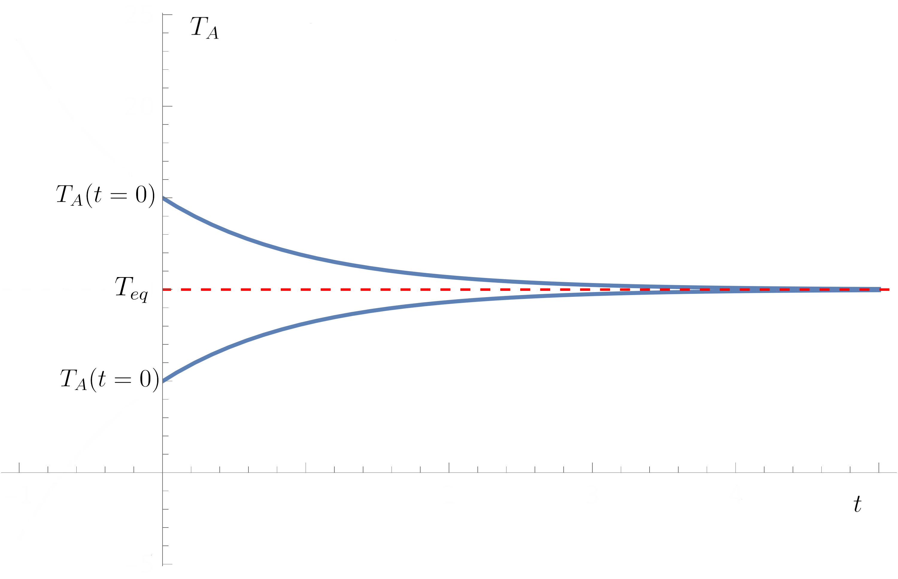
We can define the steady-state solution (also known as constant equilibrium solution) by assuming , to obtain
The ordinary differential equation (2) can be recast into
and solved analytically as
where and is the initial temperature of the system.
For large times, , the term , which shows that the solution will get to an equilibrium for large times. Depending on the choice of , we will converge to from below or from above:
Created by Gregor Gassner and Andrés Rueda-Ramírez with contributions by Simone Chiocchetti, Daniel Bach, Sophia Horak, Philipp Baasch, Benjamin Bolm, Erik Faulhaber, and Luca Sommer. Last modified: April 02, 2026. Website built with Franklin.jl and the Julia programming language.