Milestone 3 - Project Results

Expected Results

This is an example for the expected results:

Solar Forcing vector

Spatial averages for every time step as a vector in a .txt file:
(Download solar_forcing_averages.txt)

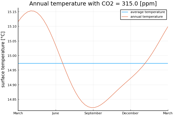
Annual Temperature Plot

Calculated with the forward Euler method. Plot for the backward Euler is almost identical.

Files Download

The Julia and Python implementations of milestone 3 can be downloaded here:

• Julia solution

• Python solution

Scripts for Milestone 3

You can also check out our Julia and Python implementations of milestone 3 in this site.

Julia implementation of milestone 3

using LinearAlgebra

include("milestone1.jl")
include("milestone2.jl")

function calc_area(geo_dat)
    nlatitude, nlongitude = size(geo_dat)
    area = zeros(nlatitude)
    delta_theta = pi / (nlatitude - 1)

    # Poles
    area[1] = area[end] = 0.5 * (1 - cos(0.5 * delta_theta))

    # Inner cells
    for j in 2:(nlatitude - 1)
        area[j] = sin(0.5 * delta_theta) * sin(delta_theta * (j - 1)) / nlongitude
    end

    return area
end

function calc_mean(data, area)
    nlatitude, nlongitude = size(data)

    mean_data = area[1] * data[1, 1] + area[end] * data[end, end]
    for i in 2:(nlatitude - 1)
        for j in 1:nlongitude
            mean_data += area[i] * data[i, j]
        end
    end

    return mean_data
end

function calc_radiative_cooling_co2(co2_concentration, co2_concentration_base=315.0,
                                    radiative_cooling_base=210.3)
    return radiative_cooling_base - 5.35 * log(co2_concentration / co2_concentration_base)
end

function timestep_euler_forward(mean_temperature, t, delta_t, mean_heat_capacity,
                                mean_solar_forcing, radiative_cooling)
    # Rearrange the energy balance equation to
    # d/dt T = f(T, t),
    # where f(T, t) = (S_sol(t) - A - BT) / C.
    # This function is the right-hand side f,
    # where t is not the time but the array index for the corresponding time.
    function rhs(mean_temp, t_)
        return (mean_solar_forcing[t_] - radiative_cooling - 2.15 * mean_temp) /
               mean_heat_capacity
    end

    # Calculate T_t = T_{t-1} + delta_t * rhs(T_{t-1}, t-1) (forward Euler).
    if t > 1
        return mean_temperature[t - 1] + delta_t * rhs(mean_temperature[t - 1], t - 1)
    else
        # In the first iteration, we access the last entry of mean_temperature.
        # Therefore, we start in each iteration with the last temperature of the previous iteration.
        ntimesteps = length(mean_temperature)
        return mean_temperature[end] + delta_t * rhs(mean_temperature[end], ntimesteps)
    end
end

function compute_equilibrium(timestep_function, mean_heat_capacity, mean_solar_forcing,
                             radiative_cooling;
                             max_iterations=100, rel_error=2e-5, verbose=true)
    # Number of time steps per year.
    ntimesteps = length(mean_solar_forcing)

    # Step size
    delta_t = 1 / ntimesteps

    # We start with a constant area-mean temperature of 0 throughout the year.
    mean_temperature = zeros(ntimesteps)
    year_avg_temperature = 0

    # Mean temperature from the previous iteration to approximate the error.
    old_mean_temperature = copy(mean_temperature)

    for i in 1:max_iterations
        for t in 1:ntimesteps
            mean_temperature[t] = timestep_function(mean_temperature, t, delta_t,
                                                    mean_heat_capacity, mean_solar_forcing,
                                                    radiative_cooling)
        end

        year_avg_temperature = sum(mean_temperature) / ntimesteps
        verbose &&
            println("Average annual temperature in iteration $i is $year_avg_temperature.")

        if norm(mean_temperature - old_mean_temperature) < rel_error
            # We can assume that the error is sufficiently small now.
            verbose && println("Equilibrium reached!")
            break
        else
            # Note that we need to write the values from mean_temperature to old_mean_temperature
            # in order to get two arrays with the same values.
            # We can't omit the [:] or we would only have one array with two pointers to it.
            old_mean_temperature[:] = mean_temperature
        end
    end

    return mean_temperature, year_avg_temperature
end

function timestep_euler_backward(mean_temperature, t, delta_t, mean_heat_capacity,
                                 mean_solar_forcing, radiative_cooling)
    # This time, we have to solve the equation
    # T_t = T_{t-1} + delta_t * f(T_t, t),
    # where f(T, t) = (S_sol(t) - A - BT) / C.
    # For this, we have to separate the terms that depend on T and the source terms that only depend on t.
    # Solving for T_t yields
    # T_t = (T_{t-1} + delta_t * (S_sol[t] - A) / C) / (1 + delta_t * B / C).
    # Note that in the first iteration, we access mean_temperature[-1], which is the last entry.
    # Therefore, we start in each iteration with the last temperature of the previous iteration.
    source_terms = (mean_solar_forcing[t] - radiative_cooling) / mean_heat_capacity

    if t > 1
        previous_mean_temperature = mean_temperature[t - 1]
    else
        previous_mean_temperature = mean_temperature[end]
    end

    return (previous_mean_temperature + delta_t * source_terms) /
           (1 + delta_t * 2.15 / mean_heat_capacity)
end

function plot_annual_temperature(annual_temperature, average_temperature, title)
    ntimesteps = length(annual_temperature)
    labels = ["March", "June", "September", "December", "March"]

    p = plot(average_temperature * ones(ntimesteps), label="average temperature",
             xlims=(1, ntimesteps), xticks=(LinRange(1, ntimesteps, 5), labels),
             ylabel="surface temperature [°C]", title=title)
    plot!(p, annual_temperature, label="annual temperature")

    return p
end

# Run code
function milestone3()
    geo_dat_ = read_geography(joinpath(@__DIR__, "input", "The_World128x65.dat"))

    albedo = calc_albedo(geo_dat_)
    heat_capacity = calc_heat_capacity(geo_dat_)

    # Compute solar forcing
    true_longitude = read_true_longitude(joinpath(@__DIR__, "input", "True_Longitude.dat"))
    solar_forcing = calc_solar_forcing(albedo, true_longitude)

    # Compute area-mean quantities
    area_ = calc_area(geo_dat_)

    mean_albedo = calc_mean(albedo, area_)
    print("Mean albedo = $mean_albedo")

    mean_heat_capacity_ = calc_mean(heat_capacity, area_)
    print("Mean heat capacity = $mean_heat_capacity_")

    ntimesteps_ = length(true_longitude)
    mean_solar_forcing_ = [calc_mean(solar_forcing[:, :, t], area_) for t in 1:ntimesteps_]

    co2_ppm = 315.0
    radiative_cooling_ = calc_radiative_cooling_co2(co2_ppm)

    # Compute and plot temperature with Euler forward
    (annual_temperature_,
     average_temperature_) = compute_equilibrium(timestep_euler_forward,
                                                 mean_heat_capacity_,
                                                 mean_solar_forcing_,
                                                 radiative_cooling_)
    plot_forward = plot_annual_temperature(annual_temperature_, average_temperature_,
                                           "Annual temperature with CO2 = $co2_ppm [ppm]")

    # Compute and plot temperature with Euler backward
    (annual_temperature_,
     average_temperature_) = compute_equilibrium(timestep_euler_backward,
                                                 mean_heat_capacity_,
                                                 mean_solar_forcing_,
                                                 radiative_cooling_)
    plot_backward = plot_annual_temperature(annual_temperature_, average_temperature_,
                                            "Annual temperature with CO2 = $co2_ppm [ppm]")

    # Show both plots
    display(plot_forward)
    display(plot_backward)

    return plot_forward, plot_backward
end

Python implementation of milestone 3

import matplotlib.pyplot as plt
import numpy as np

from milestone1 import read_geography
from milestone2 import calc_albedo, calc_heat_capacity, calc_solar_forcing, read_true_longitude


def calc_area(geo_dat):
    nlatitude, nlongitude = geo_dat.shape
    area = np.zeros(nlatitude, dtype=np.float64)
    delta_theta = np.pi / (nlatitude - 1)

    # Poles
    area[0] = area[-1] = 0.5 * (1 - np.cos(0.5 * delta_theta))

    # Inner cells
    for j in range(1, nlatitude - 1):
        area[j] = np.sin(0.5 * delta_theta) * np.sin(delta_theta * j) / nlongitude

    return area


def calc_mean(data, area):
    nlatitude, nlongitude = data.shape

    mean_data = area[0] * data[0, 0] + area[-1] * data[-1, -1]
    for i in range(1, nlatitude - 1):
        for j in range(nlongitude):
            mean_data += area[i] * data[i, j]

    return mean_data


def calc_radiative_cooling_co2(co2_concentration, co2_concentration_base=315.0,
                               radiative_cooling_base=210.3):
    return radiative_cooling_base - 5.35 * np.log(co2_concentration / co2_concentration_base)


def timestep_euler_forward(mean_temperature, t, delta_t, mean_heat_capacity, mean_solar_forcing, radiative_cooling):
    # Rearrange the energy balance equation to
    # d/dt T = f(T, t),
    # where f(T, t) = (S_sol(t) - A - BT) / C.
    # This function is the right-hand side f,
    # where t is not the time but the array index for the corresponding time.
    def rhs(mean_temp, t_):
        return (mean_solar_forcing[t_] - radiative_cooling - 2.15 * mean_temp) / mean_heat_capacity

    # Calculate T_t = T_{t-1} + delta_t * rhs(T_{t-1}, t-1) (forward Euler).
    # Note that in the first iteration, we access mean_temperature[-1], which is the last entry.
    # Therefore, we start in each iteration with the last temperature of the previous iteration.
    return mean_temperature[t - 1] + delta_t * rhs(mean_temperature[t - 1], t - 1)


def compute_equilibrium(timestep_function, mean_heat_capacity, mean_solar_forcing, radiative_cooling,
                        max_iterations=100, rel_error=2e-5, verbose=True):
    # Number of time steps per year.
    ntimesteps = len(mean_solar_forcing)

    # Step size
    delta_t = 1 / ntimesteps

    # We start with a constant area-mean temperature of 0 throughout the year.
    mean_temperature = np.zeros(ntimesteps)
    year_avg_temperature = 0

    # Mean temperature from the previous iteration to approximate the error.
    old_mean_temperature = np.copy(mean_temperature)

    for i in range(max_iterations):
        for t in range(ntimesteps):
            mean_temperature[t] = timestep_function(mean_temperature, t, delta_t,
                                                    mean_heat_capacity, mean_solar_forcing, radiative_cooling)

        year_avg_temperature = np.sum(mean_temperature) / ntimesteps
        verbose and print(f"Average annual temperature in iteration {i} is {year_avg_temperature}.")

        if np.linalg.norm(mean_temperature - old_mean_temperature) < rel_error:
            # We can assume that the error is sufficiently small now.
            verbose and print("Equilibrium reached!")
            break
        else:
            # Note that we need to write the values from mean_temperature to old_mean_temperature
            # in order to get two arrays with the same values.
            # We can't omit the [:] or we would only have one array with two pointers to it.
            old_mean_temperature[:] = mean_temperature

    return mean_temperature, year_avg_temperature


def timestep_euler_backward(mean_temperature, t, delta_t, mean_heat_capacity, mean_solar_forcing, radiative_cooling):
    # This time, we have to solve the equation
    # T_t = T_{t-1} + delta_t * f(T_t, t),
    # where f(T, t) = (S_sol(t) - A - BT) / C.
    # For this, we have to separate the terms that depend on T and the source terms that only depend on t.
    # Solving for T_t yields
    # T_t = (T_{t-1} + delta_t * (S_sol[t] - A) / C) / (1 + delta_t * B / C).
    # Note that in the first iteration, we access mean_temperature[-1], which is the last entry.
    # Therefore, we start in each iteration with the last temperature of the previous iteration.
    source_terms = (mean_solar_forcing[t] - radiative_cooling) / mean_heat_capacity

    return (mean_temperature[t - 1] + delta_t * source_terms) / (1 + delta_t * 2.15 / mean_heat_capacity)


def plot_annual_temperature(annual_temperature, average_temperature, title):
    fig, ax = plt.subplots()

    ntimesteps = len(annual_temperature)
    plt.plot(average_temperature * np.ones(ntimesteps), label="average temperature")
    plt.plot(annual_temperature, label="annual temperature")

    plt.xlim((0, ntimesteps - 1))
    labels = ["March", "June", "September", "December", "March"]
    plt.xticks(np.linspace(0, ntimesteps - 1, 5), labels)
    ax.set_ylabel("surface temperature [°C]")
    plt.grid()
    plt.title(title)
    plt.legend(loc="upper right")

    plt.tight_layout()
    plt.show()


# Run code
if __name__ == "__main__":
    geo_dat_ = read_geography("input/The_World128x65.dat")

    albedo = calc_albedo(geo_dat_)
    heat_capacity = calc_heat_capacity(geo_dat_)

    # Compute solar forcing
    true_longitude = read_true_longitude("input/True_Longitude.dat")
    solar_forcing = calc_solar_forcing(albedo, true_longitude)

    # Compute area-mean quantities
    area_ = calc_area(geo_dat_)

    mean_albedo = calc_mean(albedo, area_)
    print(f"Mean albedo = {mean_albedo}")

    mean_heat_capacity_ = calc_mean(heat_capacity, area_)
    print(f"Mean heat capacity = {mean_heat_capacity_}")

    ntimesteps_ = len(true_longitude)
    mean_solar_forcing_ = [calc_mean(solar_forcing[:, :, t], area_) for t in range(ntimesteps_)]

    co2_ppm = 315.0
    radiative_cooling_ = calc_radiative_cooling_co2(co2_ppm)

    # Compute and plot temperature with Euler forward
    annual_temperature_, average_temperature_ = compute_equilibrium(timestep_euler_forward,
                                                                    mean_heat_capacity_, mean_solar_forcing_,
                                                                    radiative_cooling_)
    plot_annual_temperature(annual_temperature_, average_temperature_, f"Annual temperature with CO2 = {co2_ppm} [ppm]")

    # Compute and plot temperature with Euler backward
    annual_temperature_, average_temperature_ = compute_equilibrium(timestep_euler_backward,
                                                                    mean_heat_capacity_, mean_solar_forcing_,
                                                                    radiative_cooling_)
    plot_annual_temperature(annual_temperature_, average_temperature_, f"Annual temperature with CO2 = {co2_ppm} [ppm]")