Milestone 4 - Multiple 0D-EBMs

As a next step, we want to actually use the local information $C(x)$, $\alpha(x)$, and $S(x,t)$ that we have available, see milestone 2. Hence, the idea for the next improvement of our 0D-EBM is to set up local ODE problems separately for each grid node $j,i$. Then solve all the ODEs for each grid node to get a full 2D temperature field (3D field, if we count the time dependence as well).

The local 0D-EBM for a local grid node $i=1, \ldots, \texttt{n\_longitude}$ and $j=1, \ldots, \texttt{n\_latitude}$ is given by

and is solved separately for each node. After solving the ODEs, we can then average the resulting time-dependent temperature field $T[j,i,k]$, over the whole globe, and/or separately for the northern and the southern hemispheres. The results are plotted in the next figure

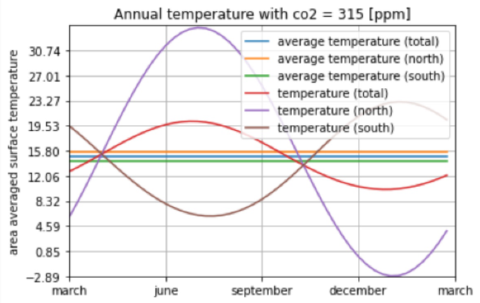
We can observe some significant changes in the quality of our approximation:

(i) The difference in the temperature variations in the North and South is much bigger now with $\Delta T_{N,max} \approx 33$ and $\Delta T_{S,max} \approx 17$ $[K]$.

(ii) Both, the North and South temperature distributions are now phase shifted compared to our 0D-EBM North-South from before. Compared to the real observed temperature distribution (and our own experience), these are much more realistic. We now can even see that the South is a bit "later" than the North, which fits our expectation because of the difference of ocean area in the South and North.

We encourage the interested reader to try out different values of $CO_2$ and to compare the data to real measured temperatures. In particular, the sensitivity of changing the $CO_2$ value and its effect on the global average temperature change $\Delta T.$

It is clear that the local 0D-EBM for each grid node has in general improved the solution quality and its physical realism. However, it is still far off from observations. In particular, the minimum and maximum temperatures seem a bit too extreme. Furthermore, the solution field appears discontinuous across strong geography changes, which is also not realistic.

As an intermediate conclusion, it seems that a major process is missing: a process that should smear out the extremes a bit (reducing minimum and maximum values) and that should also connect the different grid node solutions with each other, such that neighbour node temperatures are somewhat continuous and to get rid of the very steep gradients across geography changes.

Such a process, such a behaviour is precisely the effect/role of diffusion and dissipation. Hence, the next step to improve our 0D-EBM approach is to move away and beyond the ODE modeling and consider a PDE by incorporating heat transfer and the heat flux, i.e., the diffusion operator $\vec{\nabla}\cdot(D(x)\,\vec{\nabla} T)$.