Milestone 4 - North/South EBM

As a next step, we want to investigate the difference of the southern and nothern hemisphere. If we visualize again the surface of Earth we see a strong difference regarding the geography:

• Earth's Surface. Blue Marble Next Generation, NASA's Goddard Space Flight Center, Reto Stockli, 2004, Public Domain.

An obvious difference is that there is more ocean area in the south and more land area in the north. This is an important difference for our EBM as the heat capacity coefficient $C(x)$ has strong variations: in particular, ocean grid cells (water) have a much larger value of $C$, which indicates that the thermodynamic time scales are much longer, which means that the ocean reacts much "slower" compared to the soil.

It is even possible to estimate the thermal radiation relaxation timescales by inspecting again the temperature depending parts of our 0D-EBM,

where a simple physical units analysis shows that the ratio of $C$ and $B$ has the units of time, i.e., seconds $[s]$ (or years, depending on the temporal scaling of $C$)

The timescale $\tau$ is the relaxation time and is about $5.9$ years for the ocean and about $5.4$ days for the land. Hence, following these arguments, we do expect to see a difference in the annual temperature distribution between south and north.

To investigate this behaviour we apply our time dependent EBM again, but not for the whole Earth. We are going to use one 0D-EBM for the southern hemisphere and one for the northern hemisphere. Hence, our goal is to get two OD-EBMs: for one we have to do area-averaging over the northern hemisphere

and for the other we have to do area-averaging over the southern hemisphere

To compute the special area averages, we remind ourselves about the computational grid and the definition of the area vector that we use to compute the area average:

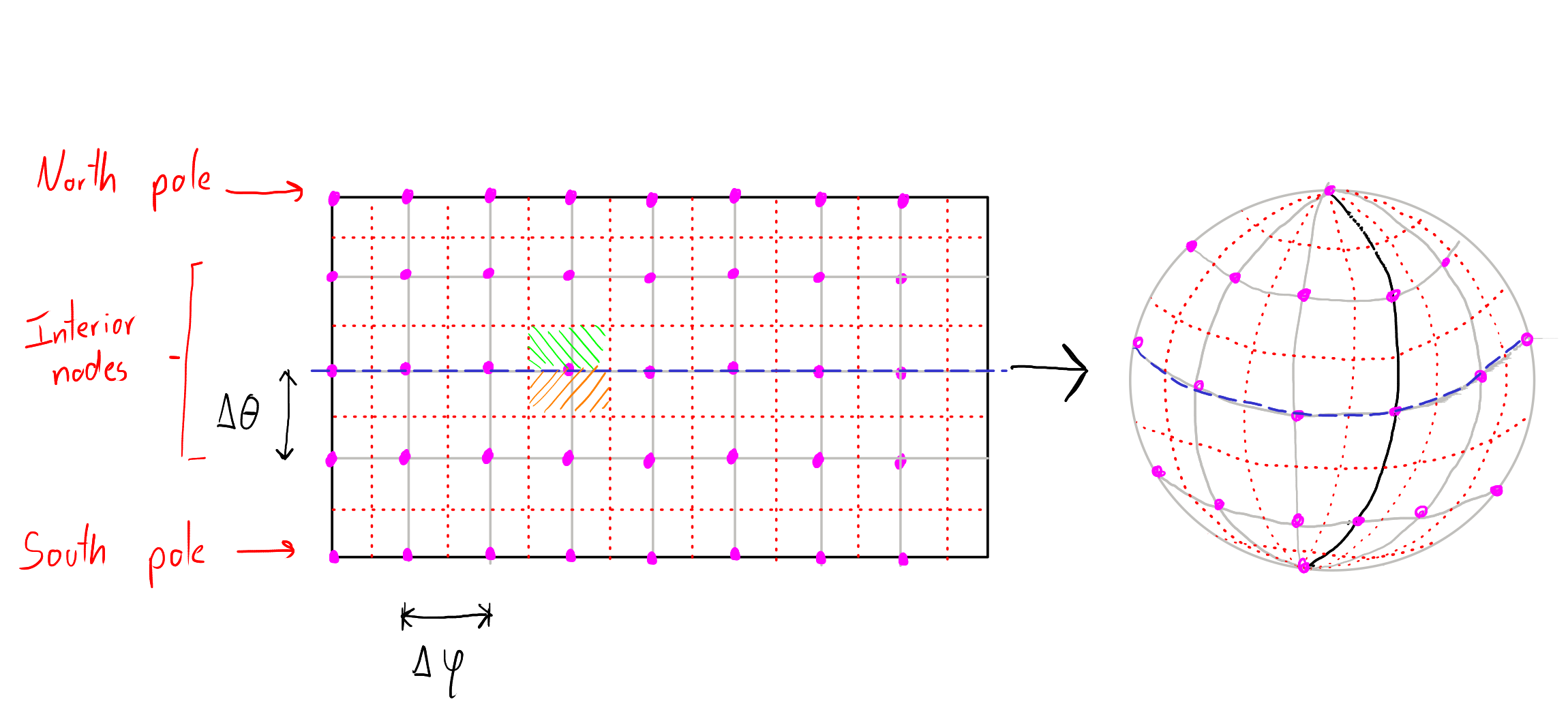
We are now marking the equator with a blue dashed line. We can see that we have to treat the grid points on the equator carefully, as their values contribute to the area averages of both the northern and southern hemispheres. If we use an odd number of points in the latitude direction, one half of the value of each equator grid cell contributes to the North and the other half to the South.

Let us assume that we have a 2D data field $F[j,i]$, with $j=1,...,\texttt{n\_latitude}$ and $i=1,...,\texttt{n\_longitude}$, for which we want to compute an area average over the nothern hemisphere. We assume that we have our area vector $area[j]$, with $j=1,...,\texttt{n\_latitude}$, from milestone 3. With the assumption that along the longitude direction $i$, all values at the north pole of $F[1,i]$ are the same, we can compute the area average as

Note that we are multiplying by the factor $2$ as our $\texttt{area}[j]$ vector is normalized for the whole sphere surface, but the North is only half of it. In an analogous way, we can easily compute the area average of the southern hemisphere.

With these new averages, and the tools we developed before, we are able to now generate a 0D-EBM for the northern and the southern hemispheres each. We solve the two 0D-EBM models individually to equilibrium as an approximation. The next figure shows the annual temperature distributsions:

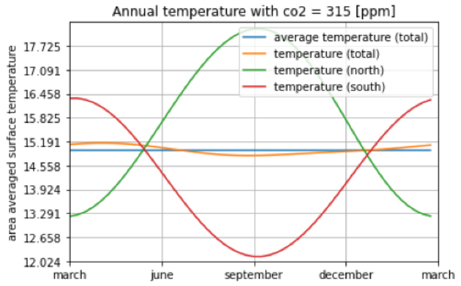
We can clearly see that the temperature distributions of north and south are phase shifted. It seems, however, that the phase shift in this simple model is mainly due to the seasonal difference of the solar insolation. There is no clear effect due to the difference in heat capacity visible. The average heat-capacities are $\overline{C}_N = 5.2$ $[J/Ksm]$ and $\overline{C}_S=7$ $[J/Ksm]$. If we check the maximum temperature variation in the hemispheres, we get $\Delta T_{N,max} = 5$ and $\Delta T_{S,max} = 4.2$ $[K]$, which shows that a lower heat-capacity allows for a stronger variation in temperature. From our own experience about the annual seasons, it is clear that the seasonal temperature distribution from both, the North and the South, are still off. It seems that averaging our EBM first in the North and in the South, then compute the temperatures is too crude of an approximation to capture the seasonal temperature distribution accurately.