Milestone 4 - Project Results

Expected Results

This is an example for the expected results:

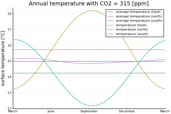
Mean Temperature Plot

Plot of the mean and average temperature calculated by averaging over the regions first and then using the 0D-EBM.

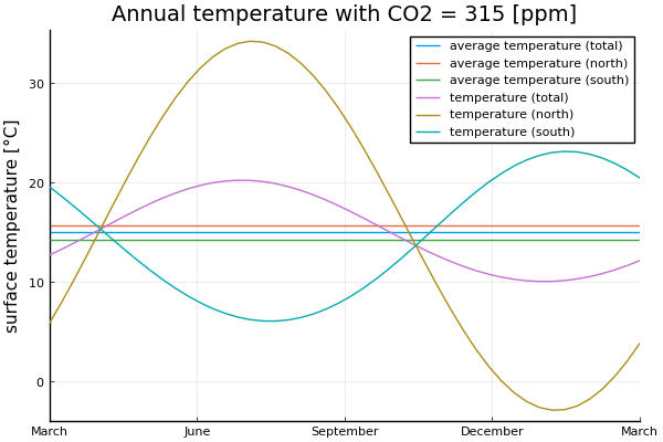
Mean Temperature Plot using Pointwise EBM

Plot of the mean and average temperature calculated by using a 0D-EBM for every point of the discretization and then averaging over the results.

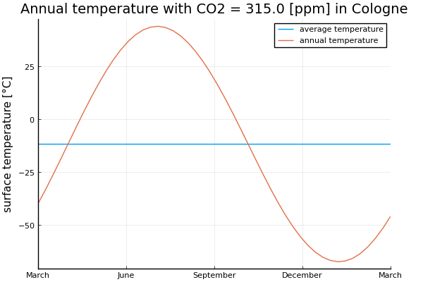
Cologne Temperature

Cologne temperature calculated via the pointwise 0D-EBM

Annual Temperature Animation

Annual temperature with the pointwise 0D-EBM:

Files Download

The Julia and Python implementations of milestone 4 can be downloaded here:

• Julia solution

• Python solution

Scripts for Milestone 4

You can also check out our Julia and Python implementations of milestone 4 in this site.

Julia implementation of milestone 4

include("milestone1.jl")
include("milestone2.jl")
include("milestone3.jl")

function calc_mean_north(data, area)
    nlatitude, nlongitude = size(data)
    j_equator = Int((nlatitude - 1) / 2) + 1

    # North Pole
    mean_data = area[1] * data[1, 1]

    # Inner nodes
    for j in 2:(j_equator - 1)
        for i in 1:nlongitude
            mean_data += area[j] * data[j, i]
        end
    end

    # Equator
    for i in 1:nlongitude
        mean_data += 0.5 * area[j_equator] * data[j_equator, i]
    end

    return 2 * mean_data
end

function calc_mean_south(data, area)
    nlatitude, nlongitude = size(data)
    j_equator = Int((nlatitude - 1) / 2) + 1

    # South Pole
    mean_data = area[end] * data[end, end]

    # Inner nodes
    for j in (j_equator + 1):(nlatitude - 1)
        for i in 1:nlongitude
            mean_data += area[j] * data[j, i]
        end
    end

    # Equator
    for i in 1:nlongitude
        mean_data += 0.5 * area[j_equator] * data[j_equator, i]
    end

    return 2 * mean_data
end

function plot_annual_temperature_north_south(annual_temperature_north,
                                             annual_temperature_south,
                                             annual_temperature_total,
                                             average_temperature_north,
                                             average_temperature_south,
                                             average_temperature_total)
    ntimesteps = length(annual_temperature_total)
    labels = ["March", "June", "September", "December", "March"]

    p = plot(average_temperature_total * ones(ntimesteps),
             label="average temperature (total)",
             xlims=(1, ntimesteps), xticks=(LinRange(1, ntimesteps, 5), labels),
             ylabel="surface temperature [°C]",
             title="Annual temperature with CO2 = 315 [ppm]")
    plot!(p, average_temperature_north * ones(ntimesteps),
          label="average temperature (north)")
    plot!(p, average_temperature_south * ones(ntimesteps),
          label="average temperature (south)")
    plot!(p, annual_temperature_total, label="temperature (total)")
    plot!(p, annual_temperature_north, label="temperature (north)")
    plot!(p, annual_temperature_south, label="temperature (south)")

    return p
end

function plot_temperature(temperature, geo_dat, timestep)
    vmin = minimum(temperature)
    vmax = -vmin # We want to have 0°C in the center.

    nlatitude, nlongitude = size(temperature)
    x, y = robinson_projection(nlatitude, nlongitude)

    ntimesteps = size(temperature, 3)
    day = (round(Int, (timestep - 1) / ntimesteps * 365) + 80) % 365
    p = contourf(x, y, temperature[:, :, timestep],
                 clims=(vmin, vmax),
                 levels=LinRange(vmin, vmax, 200),
                 aspect_ratio=1,
                 title="Temperature for Day $day",
                 c=:seismic,
                 colorbar_title="temperature [°C]",
                 axis=([], false),
                 dpi=300)

    # Add contour lines
    contour!(p, x, y, geo_dat, levels=[0.5, 1.5, 2.5, 3.5, 6.5],
             color=[:black], linewidth=0.6)

    return p
end

# Run code
function milestone4()
    geo_dat = read_geography(joinpath(@__DIR__, "input", "The_World128x65.dat"))
    nlatitude, nlongitude = size(geo_dat)

    albedo = calc_albedo(geo_dat)
    heat_capacity = calc_heat_capacity(geo_dat)

    # Compute solar forcing
    true_longitude = read_true_longitude(joinpath(@__DIR__, "input", "True_Longitude.dat"))
    solar_forcing = calc_solar_forcing(albedo, true_longitude)

    # Compute area-mean quantities
    area = calc_area(geo_dat)

    mean_albedo_north = calc_mean_north(albedo, area)
    print("Mean albedo north = $mean_albedo_north")
    mean_albedo_south = calc_mean_south(albedo, area)
    print("Mean albedo south = $mean_albedo_south")
    mean_albedo_total = calc_mean(albedo, area)
    print("Mean albedo total = $mean_albedo_total")

    mean_heat_capacity_north = calc_mean_north(heat_capacity, area)
    print("Mean heat capacity north = $mean_heat_capacity_north")
    mean_heat_capacity_south = calc_mean_south(heat_capacity, area)
    print("Mean heat capacity south = $mean_heat_capacity_south")
    mean_heat_capacity_total = calc_mean(heat_capacity, area)
    print("Mean heat capacity total = $mean_heat_capacity_total")

    ntimesteps = length(true_longitude)
    mean_solar_forcing_north = [calc_mean_north(solar_forcing[:, :, t], area)
                                for t in 1:ntimesteps]
    mean_solar_forcing_south = [calc_mean_south(solar_forcing[:, :, t], area)
                                for t in 1:ntimesteps]
    mean_solar_forcing_total = [calc_mean(solar_forcing[:, :, t], area)
                                for t in 1:ntimesteps]

    co2_ppm = 315.0
    radiative_cooling = calc_radiative_cooling_co2(co2_ppm)

    # Compute equilibrium for all three means
    (annual_temperature_north_,
     average_temperature_north_) = compute_equilibrium(timestep_euler_forward,
                                                       mean_heat_capacity_north,
                                                       mean_solar_forcing_north,
                                                       radiative_cooling)
    (annual_temperature_south_,
     average_temperature_south_) = compute_equilibrium(timestep_euler_forward,
                                                       mean_heat_capacity_south,
                                                       mean_solar_forcing_south,
                                                       radiative_cooling)
    (annual_temperature_total_,
     average_temperature_total_) = compute_equilibrium(timestep_euler_forward,
                                                       mean_heat_capacity_total,
                                                       mean_solar_forcing_total,
                                                       radiative_cooling)

    plot_mean = plot_annual_temperature_north_south(annual_temperature_north_,
                                                    annual_temperature_south_,
                                                    annual_temperature_total_,
                                                    average_temperature_north_,
                                                    average_temperature_south_,
                                                    average_temperature_total_)

    # Calculate annual temperature for every grid point
    annual_temperature_pointwise = Array{Float64, 3}(undef, nlatitude, nlongitude,
                                                     ntimesteps)
    for j in 1:nlongitude, i in 1:nlatitude
        # I/O in Julia is pretty slow, so this takes forever with `verbose=true`.
        (annual_temperature,
         _) = compute_equilibrium(timestep_euler_forward,
                                  heat_capacity[i, j],
                                  solar_forcing[i, j, :],
                                  radiative_cooling,
                                  verbose=false)

        annual_temperature_pointwise[i, j, :] = annual_temperature
    end

    # Area mean of pointwise annual temperature
    annual_mean_temperature_north = [calc_mean_north(annual_temperature_pointwise[:, :, t],
                                                     area)
                                     for t in 1:ntimesteps]
    annual_mean_temperature_south = [calc_mean_south(annual_temperature_pointwise[:, :, t],
                                                     area)
                                     for t in 1:ntimesteps]
    annual_mean_temperature_total = [calc_mean(annual_temperature_pointwise[:, :, t], area)
                                     for t in 1:ntimesteps]

    average_temperature_north_ = sum(annual_mean_temperature_north) / ntimesteps
    average_temperature_south_ = sum(annual_mean_temperature_south) / ntimesteps
    average_temperature_total_ = sum(annual_mean_temperature_total) / ntimesteps

    plot_pointwise = plot_annual_temperature_north_south(annual_mean_temperature_north,
                                                         annual_mean_temperature_south,
                                                         annual_mean_temperature_total,
                                                         average_temperature_north_,
                                                         average_temperature_south_,
                                                         average_temperature_total_)

    # Compute temperature in Cologne.
    # Cologne lies about halfway between these two grid points.
    annual_temperature_cologne = (annual_temperature_pointwise[15, 68, :] +
                                  annual_temperature_pointwise[15, 69, :]) / 2
    average_temperature_cologne = sum(annual_temperature_cologne) / ntimesteps

    plot_cologne = plot_annual_temperature(annual_temperature_cologne,
                                           average_temperature_cologne,
                                           "Annual temperature with CO2 = $co2_ppm [ppm] in Cologne")

    # Animate annual temperature
    anim = @animate for ts in 1:ntimesteps
        plot_temperature(annual_temperature_pointwise, geo_dat, ts)
    end

    plot_temperature_day_80 = plot_temperature(annual_temperature_pointwise, geo_dat, 1)
    gif_annual_temperature = gif(anim, joinpath(@__DIR__, "annual_temperature.gif"), fps=7)

    # Show all plots and the animation
    display(plot_mean)
    display(plot_pointwise)
    display(plot_cologne)
    display(gif_annual_temperature)

    return plot_mean, plot_pointwise, plot_cologne, plot_temperature_day_80,
           gif_annual_temperature
end

Python implementation of milestone 4

import os

import imageio
import matplotlib.colors as colors
import matplotlib.pyplot as plt
import numpy as np

from milestone1 import read_geography, robinson_projection
from milestone2 import read_true_longitude
from milestone3 import calc_area, calc_albedo, calc_solar_forcing, calc_mean, calc_heat_capacity, \
    calc_radiative_cooling_co2, compute_equilibrium, timestep_euler_forward, plot_annual_temperature


def calc_mean_north(data, area):
    nlatitude, nlongitude = data.shape
    j_equator = int((nlatitude - 1) / 2)

    # North Pole
    mean_data = area[0] * data[0, 0]

    # Inner nodes
    for j in range(1, j_equator):
        for i in range(nlongitude):
            mean_data += area[j] * data[j, i]

    # Equator
    for i in range(nlongitude):
        mean_data += 0.5 * area[j_equator] * data[j_equator, i]

    return 2 * mean_data


def calc_mean_south(data, area):
    nlatitude, nlongitude = data.shape
    j_equator = int((nlatitude - 1) / 2)

    # South Pole
    mean_data = area[-1] * data[-1, -1]

    # Inner nodes
    for j in range(j_equator + 1, nlatitude - 1):
        for i in range(nlongitude):
            mean_data += area[j] * data[j, i]

    # Equator
    for i in range(nlongitude):
        mean_data += 0.5 * area[j_equator] * data[j_equator, i]

    return 2 * mean_data


def plot_annual_temperature_north_south(annual_temperature_north, annual_temperature_south, annual_temperature_total,
                                        average_temperature_north, average_temperature_south,
                                        average_temperature_total):
    fig, ax = plt.subplots()

    ntimesteps = len(annual_temperature_total)
    plt.plot(average_temperature_total * np.ones(ntimesteps), label="average temperature (total)")
    plt.plot(average_temperature_north * np.ones(ntimesteps), label="average temperature (north)")
    plt.plot(average_temperature_south * np.ones(ntimesteps), label="average temperature (south)")
    plt.plot(annual_temperature_total, label="temperature (total)")
    plt.plot(annual_temperature_north, label="temperature (north)")
    plt.plot(annual_temperature_south, label="temperature (south)")

    plt.xlim((0, ntimesteps - 1))
    labels = ["March", "June", "September", "December", "March"]
    plt.xticks(np.linspace(0, ntimesteps - 1, 5), labels)
    ax.set_ylabel("surface temperature [°C]")
    plt.grid()
    plt.title(f"Annual temperature with CO2 = 315 [ppm]")
    plt.legend(loc="upper right")

    plt.tight_layout()
    plt.show()


# Similar to plot_robinson_projection in MS1, but we also add contour lines
def plot_robinson_projection_with_lines(data, geo_dat, title, **kwargs):
    # Get the coordinates for the Robinson projection.
    nlatitude, nlongitude = data.shape
    x, y = robinson_projection(nlatitude, nlongitude)

    # Start plotting.
    fig, ax = plt.subplots()

    # Create contour plot of geography information against x and y.
    im = ax.contourf(x, y, data, **kwargs)

    # Add contour lines with levels from MS1
    levels = [0.5, 1.5, 2.5, 3.5, 6.5]
    ax.contour(x, y, geo_dat, colors="black", linewidths=0.6, levels=levels, linestyles="solid")

    plt.title(title)
    ax.set_aspect("equal")

    # Remove axes and ticks.
    plt.xticks([])
    plt.yticks([])
    ax.spines["top"].set_visible(False)
    ax.spines["right"].set_visible(False)
    ax.spines["bottom"].set_visible(False)
    ax.spines["left"].set_visible(False)

    # Colorbar with the same height as the plot. Code copied from
    # https://stackoverflow.com/a/18195921
    # create an axes on the right side of ax. The width of cax will be 5%
    # of ax and the padding between cax and ax will be fixed at 0.05 inch.
    from mpl_toolkits.axes_grid1 import make_axes_locatable
    divider = make_axes_locatable(ax)
    cax = divider.append_axes("right", size="5%", pad=0.05)
    cbar = plt.colorbar(im, cax=cax)

    return cbar


def plot_temperature(temperature, geo_dat, timestep, show_plot=False):
    vmin = np.amin(temperature)
    vmax = np.amax(temperature)
    levels = np.linspace(vmin, vmax, 200)
    norm = colors.TwoSlopeNorm(vmin=vmin, vcenter=0, vmax=vmax)

    # Reuse plotting function from milestone 1.
    ntimesteps = temperature.shape[2]
    day = (np.int_(timestep / ntimesteps * 365) + 80) % 365
    cbar = plot_robinson_projection_with_lines(temperature[:, :, timestep], geo_dat,
                                               f"Temperature for Day {day}",
                                               levels=levels, cmap="seismic",
                                               vmin=vmin, vmax=vmax, norm=norm)
    cbar.set_label("surface temperature [°C]")

    # Adjust size of plot to viewport to prevent clipping of the legend.
    plt.tight_layout()

    filename = f"temperature_{timestep}.png"
    plt.savefig(filename, dpi=300)
    if show_plot:
        plt.show()
    plt.close()

    return filename


# Run code
if __name__ == '__main__':
    geo_dat_ = read_geography("input/The_World128x65.dat")
    nlatitude_, nlongitude_ = geo_dat_.shape

    albedo = calc_albedo(geo_dat_)
    heat_capacity = calc_heat_capacity(geo_dat_)

    # Compute solar forcing
    true_longitude = read_true_longitude("input/True_Longitude.dat")
    solar_forcing = calc_solar_forcing(albedo, true_longitude)

    # Compute area-mean quantities
    area_ = calc_area(geo_dat_)

    mean_albedo_north = calc_mean_north(albedo, area_)
    print(f"Mean albedo north = {mean_albedo_north}")
    mean_albedo_south = calc_mean_south(albedo, area_)
    print(f"Mean albedo south = {mean_albedo_south}")
    mean_albedo_total = calc_mean(albedo, area_)
    print(f"Mean albedo total = {mean_albedo_total}")

    mean_heat_capacity_north = calc_mean_north(heat_capacity, area_)
    print(f"Mean heat capacity north = {mean_heat_capacity_north}")
    mean_heat_capacity_south = calc_mean_south(heat_capacity, area_)
    print(f"Mean heat capacity south = {mean_heat_capacity_south}")
    mean_heat_capacity_total = calc_mean(heat_capacity, area_)
    print(f"Mean heat capacity total = {mean_heat_capacity_total}")

    ntimesteps_ = len(true_longitude)
    mean_solar_forcing_north = [calc_mean_north(solar_forcing[:, :, t], area_) for t in range(ntimesteps_)]
    mean_solar_forcing_south = [calc_mean_south(solar_forcing[:, :, t], area_) for t in range(ntimesteps_)]
    mean_solar_forcing_total = [calc_mean(solar_forcing[:, :, t], area_) for t in range(ntimesteps_)]

    co2_ppm = 315.0
    radiative_cooling = calc_radiative_cooling_co2(co2_ppm)

    # Compute equilibrium for all three means
    annual_temperature_north_, average_temperature_north_ = compute_equilibrium(timestep_euler_forward,
                                                                                mean_heat_capacity_north,
                                                                                mean_solar_forcing_north,
                                                                                radiative_cooling)
    annual_temperature_south_, average_temperature_south_ = compute_equilibrium(timestep_euler_forward,
                                                                                mean_heat_capacity_south,
                                                                                mean_solar_forcing_south,
                                                                                radiative_cooling)
    annual_temperature_total_, average_temperature_total_ = compute_equilibrium(timestep_euler_forward,
                                                                                mean_heat_capacity_total,
                                                                                mean_solar_forcing_total,
                                                                                radiative_cooling)

    plot_annual_temperature_north_south(annual_temperature_north_, annual_temperature_south_, annual_temperature_total_,
                                        average_temperature_north_, average_temperature_south_,
                                        average_temperature_total_)

    # Calculate annual temperature for every grid point
    def annual_temp(i, j):
        annual_temperature, _ = compute_equilibrium(timestep_euler_forward, heat_capacity[i, j],
                                                    solar_forcing[i, j, :], radiative_cooling,
                                                    verbose=False)

        return annual_temperature

    annual_temperature_pointwise = np.array(
        [[annual_temp(i, j) for j in range(nlongitude_)] for i in range(nlatitude_)])

    # Area mean of pointwise annual temperature
    annual_mean_temperature_north = [calc_mean_north(annual_temperature_pointwise[:, :, t], area_)
                                     for t in range(ntimesteps_)]
    annual_mean_temperature_south = [calc_mean_south(annual_temperature_pointwise[:, :, t], area_)
                                     for t in range(ntimesteps_)]
    annual_mean_temperature_total = [calc_mean(annual_temperature_pointwise[:, :, t], area_)
                                     for t in range(ntimesteps_)]

    average_temperature_north_ = np.sum(annual_mean_temperature_north) / ntimesteps_
    average_temperature_south_ = np.sum(annual_mean_temperature_south) / ntimesteps_
    average_temperature_total_ = np.sum(annual_mean_temperature_total) / ntimesteps_

    plot_annual_temperature_north_south(annual_mean_temperature_north, annual_mean_temperature_south,
                                        annual_mean_temperature_total, average_temperature_north_,
                                        average_temperature_south_, average_temperature_total_)

    # Compute temperature in Cologne.
    # Cologne lies about halfway between these two grid points.
    annual_temperature_cologne = (annual_temperature_pointwise[14, 67, :] +
                                  annual_temperature_pointwise[14, 68, :]) / 2
    average_temperature_cologne = np.sum(annual_temperature_cologne) / ntimesteps_

    plot_annual_temperature(annual_temperature_cologne, average_temperature_cologne,
                            f"Annual temperature with CO2 = {co2_ppm} [ppm] in Cologne")

    # Plot temperature for each time step
    filenames = []
    for ts in range(ntimesteps_):
        filename_ = plot_temperature(annual_temperature_pointwise, geo_dat_, ts, show_plot=False)
        filenames.append(filename_)

    # Build GIF
    frames = [imageio.v3.imread(filename_) for filename_ in filenames]
    imageio.mimsave("annual_temperature.gif", frames)

    # Remove files
    for filename_ in set(filenames):
        os.remove(filename_)