Milestone 5 - Planetary Heat Transfer
Transport in the Atmosphere and Oceans
As a next improvement of our EBM, we want to connect the temperatures of the each individual grid cell to form a globally coupled system that models a smooth surface temperature field of the whole Earth. If we consider a fully coupled system where all grid cells are connected (and not independently solved as tested in milestone 4), heat will get transported from warm regions to colder regions, i.e., heat will be transported polewards. The distribution of the solar forcing term clearly shows that there is more net solar radiation in tropical latitudes than in the polar regions. Thus, some heat transfer polewards is expected. On Earth, the atmosphere and the oceans include mechanisms and processes that cause such a poleward heat transport. For the interested reader, we refer for instance to the following introductory videos that discuss some of the important processes.
Global atmospheric circulation on Earth
Effect of Coreolis force in large-scale vortices
An important property of moving fluid flows is turbulent motion. Most flows in nature (and engineering) are turbulent, which means multiscale in space and time. From very small eddies in the range of milimeters up to large vortical structures of size hundreds or thousands of meters. Turbulent flows are highly sensitive to small scale disturbances (this is known as the butterfly effect), almost chaotic and thus hard to predict. One of the very important mechanisms of turbulent flows is increased mixing efficiency of cold and warm fluids, i.e., an enhanced heat transfer and heat distribution. This formally requires the numerical resolution (very small grid cells) of all small and large eddies. Small grid cells of course make the simulations very computationally intense and unfortunately for realistic flow scenarios too expensive, even on today's largest super computers. Hence, the full resolution of turbulent fluids is an unsolved problem in fluid mechanics. The current strategy in computational fluid dynamics (and also atmospheric science) to deal with this problem is to introduce additional parametrizations (also often coined turbulence models) that account for the effects of small eddies that cannot be resolved by the grid, so-called subgrid effects. Hence, all modern ESM include a full atmosphere simulation model, which itself includes parametrization for subgrid scale turbulence.
Modeling Turbulent and Polewards Heat Transport with Diffusion
In his pioneering work, Budyko
considered a simple 1D (latitude dependent) EBM that included a simple term that models heat transfer accross latitude zones. From satellite data one can reconstruct that the main heat transfer depends on the latitude and is polewards. The next figure, for instance, shows the heat transfer in the northern hemisphere. It is also worth noting that the heat transfer in the atmosphere is different compared to the ocean.
Heat transfer in the northern hemisphere. Generated with data from "Maslin (2013). 'Climate: A Very Short Introduction'"
The idea of Budyko was to include an algebraic term that is proportional to
where is the temperature at latitude , is the mean global surface temperature, and is a parameter that can be adjusted. The next figure shows a sketch of the model with energy fluxes across the latitude zones (rings), where the coefficient is denoted with in this figure.
Sellers,
proposed a model for the heat transport that is based on a diffusion operator. Diffusion or heat conduction is a model where the heat flux is proportional to the gradient of the temperature
and the diffusion operator is of the form
where is now the so-called diffusion coefficient. The diffusion coefficient needs to include the effect of oceanic heat transport, turbulent mixing, the sensible heat transport and the latent heat transport. Sensible heat transfer occurs when objects with different temperatures are in direct contact (e.g. surface of the land with the atmosphere) and exchange heat. Latent heat cannot be measured directly, but is an important form of heat transfer that is relevant when a material changes its state (from liquid to gas or from ice to liquid).
Remark: It is clear that all these complex processes cannot be phenomenologically modeled by a single parameter . Coming back to our discussion on the different modeling strategies, we already had models based on first principles. These models are (supposed to be) universally valid and based on fundamental laws of nature with no tunable parameters. A next step was to approximate processes that can be measured with simplified models. These empirical models are tuned with parameters to approximate the behavior of the processes observed in measurements. The empircal models are still grounded in reality as they are calibrated with measurements, but include some for of parameter tuning. As an example, we had the radiation model of Budyko in milestone 2.
Due to the complexity of the heat transport and the many mechanisms and processes involved, we do not consider first principle modeling, nor empirical models for the heat transfer in our EBM. Instead, we resort now to another strategy in modeling. We add a simple replacement model, which does not directly mimic the processes, but mimics the effect of the processes on the solution of the EBM. To be precise, we aim to model the effect of the poleward heat transfer on the resulting EBM temperature. This simple replacement model has again parameters, which cannot be tuned to measurements and observations of processes. Instead, the idea is to tune the parameters of the model such, that the resulting solution of the model (the surface temperature) behaves as realistic as possible.
It is important to understand that this type of modeling is driven by data of the desired solution (temperature distribution), i.e., we fit the model to existing solutions (for instance from observations) as good as possible. So we do not tune the model of the process, but tune the outcome of the whole model. It is thus clear that such type of modeling is highly heuristic and should be used with extreme caution, as its predictive power is hard to gauge, i.e., expert knowledge and validation is necessary to give such an approach credibility.
Diffusion Operator in Spherical Coordinates
As we solve our EBM on the surface of Earth, i.e., in spherical coordinates, we need to define the gradient operators and the divergence operators in our natural coordinate system.
The gradient and divergence operators defined in Cartesian coordiates read as,
where is a scalar field, , , and are the unit vectors in the , , and directions, respectively, and is a vector field.
We can transform the gradient and divergence operators to the spherical coordinate system by computing the relation between the unit vectors and partial derivatives of both coordinate systems.
For instance, for the unit vectors we have
and for the partial derivatives we have
Inserting (5) and (6) into (4), we obtain the gradient and divergence operators in spherical coordinates,
The gradient operator is also commonly written in the vector form as
We obtain the diffusion operator in spherical coordinates by combining the expressions for the gradient and divergence operators to obtain
Note that these derivations are in full three-dimensional space. However, in our EBM, we consider only the surface of the Earth, i.e. a approximation of the surface temperature with the choice of the radius coordinate . Hence, heat transfer in vertical direction (along the radial coordinate ) is neglected and only the variations in latitude and longitude directions are considered. Furthermore, we absorb the scaling with the Earth radius into the diffusion coefficient and simplify the expression to obtain
Choice of the Diffusion Coefficient in the 2D EBM
Our final form of the EBM with heat diffusion reads as
respectively, in spherical coordinates
As discussed above, the heat diffusion term needs to model the complex mechanism of poleward transport of heat. There are many different choices of available in literature, from simple global constant values to more complex approximations. Here, again, we follow the paper by Zhuang et al.
We distinguish between oceanic heat transport and heat transport over land and snow/ice covered areas. We also account for a difference of the heat transfer in the northern and southern hemisphere due to the asymmetric distribution and sizes of the land masses. The following figure shows a sketch of the energy fluxes due to heat transfer accounted in our model (here, the diffusion coefficients are denoted with instead of )
Figure from TransEBM v. 1.0: description, tuning, and validation of a transient model of the Earth's energy balance in two dimensions by Elisa Ziegler and Kira Rehfeld, CC-BY 4.0.
Thus, for the actual values of the diffusion coefficients we differentiate between grid cells that represent ocean, and all other types. Furthermore, for non oceanic grid cells, we differentiate if we are in the northern or southern hemisphere.
The values for oceanic grid cells in physical unit are
with and .
The values for non oceanic grid cells in the northern hemisphere in physical units are
with and .
The values for non oceanic grid cells in the southern hemisphere in physical units are
with and .
Remark: We stress again, that the choice of the diffusion coefficients is kind of arbitrary and highly tuned to fit the resulting temperature fields as good as possible. Thus, the choice of a ramp up function between the values at the equator and the values at the poles proportional to has no deeper meaning but is a modeling/tuning choice. The resulting distribution of the diffusion coefficients over ocean and non oceanic grid cells is shown in the following figure
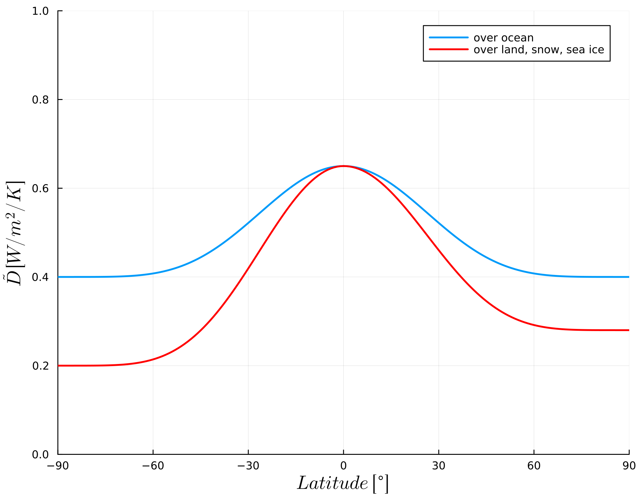
Note that this plot is showing the latitude rather than the colatitude.
Created by Gregor Gassner and Andrés Rueda-Ramírez with contributions by Simone Chiocchetti, Daniel Bach, Sophia Horak, Philipp Baasch, Benjamin Bolm, Erik Faulhaber, and Luca Sommer. Last modified: April 02, 2026. Website built with Franklin.jl and the Julia programming language.