Milestone 5 - Project Results
Expected Results
This is an example for the expected results:
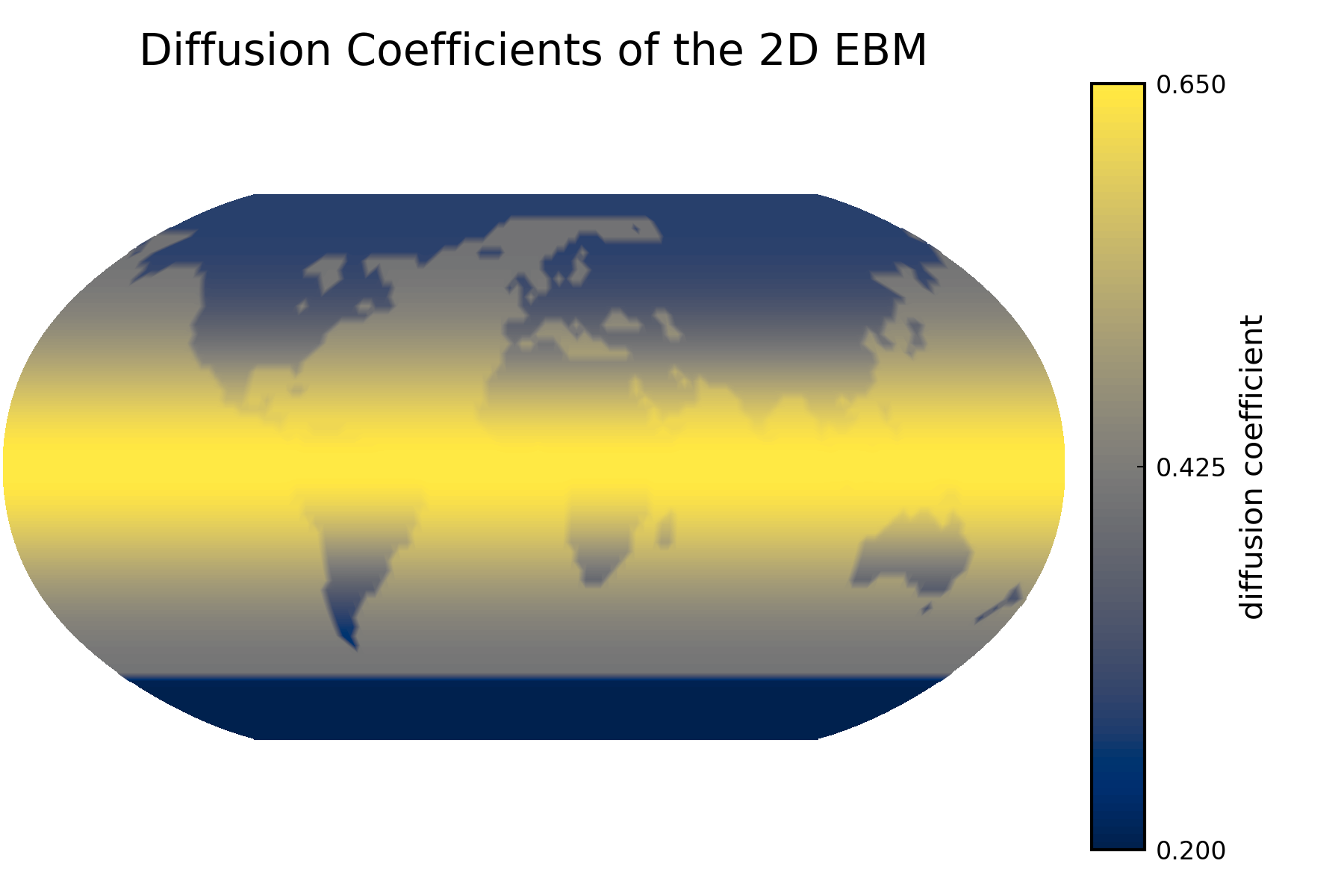
Diffusion Coefficient Plot
Plot of the diffusion coefficient:
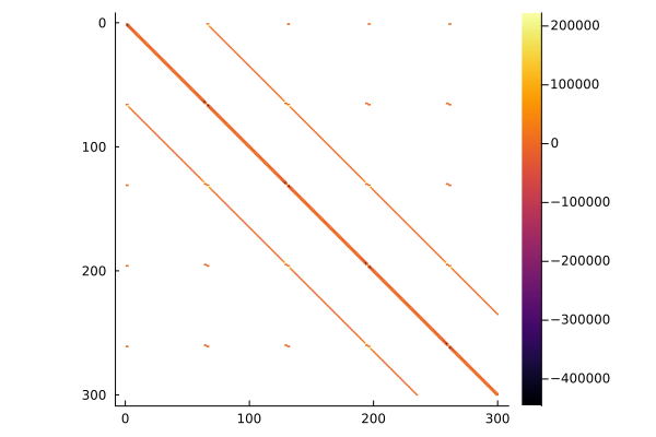
Sparsity Pattern of the Jacobian
Plot of the upper left corner of the sparsity pattern of the Jacobian. Only a the upper left part is plotted to make the pattern visible.
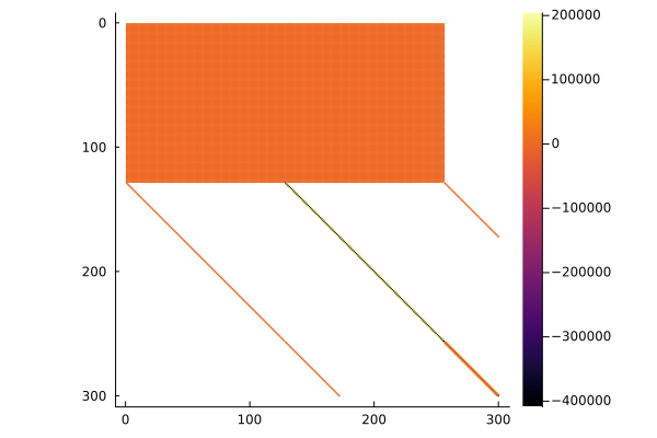
In a row-major language like Python, the sparsity pattern looks different:
⚠ Warning!
We strongly suggest to first work on the solutions on your own/within your group without checking directly for the reference solutions.
Files Download
The Python implementation of milestone 5 can be downloaded here (Julia version will be added soon):
Bonus - 3D plot
3D plot generated by Chong-Son Dröge, Fabian Höck, and Luca Levent Sommer.
Scripts for Milestone 5
You can also check out our Julia and Python implementations of milestone 5 in this site.
Julia implementation of milestone 5
include("milestone1.jl")
include("milestone2.jl")
include("milestone3.jl")

using Arpack: eigs

struct Mesh
    n_latitude::Int
    n_longitude::Int
    ndof::Int
    h::Float64
    area::Vector{Float64}
    geom::Float64
    csc2::Vector{Float64}
    cot::Vector{Float64}

    function Mesh(geo_dat)
        n_latitude, n_longitude = size(geo_dat)
        ndof = n_latitude * n_longitude
        h = pi / (n_latitude - 1)

        area = calc_area(geo_dat)
        geom = sin(0.5 * h) / area[1]

        csc2 = [1 / sin(h * (j - 1))^2 for j in 2:(n_latitude - 1)]
        cot = [1 / tan(h * (j - 1)) for j in 2:(n_latitude - 1)]

        return new(n_latitude, n_longitude, ndof, h, area, geom, csc2, cot)
    end
end

function calc_diffusion_coefficients(geo_dat)
    nlatitude, nlongitude = size(geo_dat)

    coeff_ocean_poles = 0.4
    coeff_ocean_equator = 0.65
    coeff_equator = 0.65
    coeff_north_pole = 0.28
    coeff_south_pole = 0.2

    function diffusion_coefficient(j, i)
        # Compute the j value of the equator
        j_equator = Int((nlatitude - 1) / 2) + 1

        theta = pi * (j - 1) / (nlatitude - 1)
        colat = sin(theta)^5

        geo = geo_dat[j, i]
        if geo == 5  # ocean
            return coeff_ocean_poles + (coeff_ocean_equator - coeff_ocean_poles) * colat
        else  # land, sea ice, etc
            if j <= j_equator  # northern hemisphere
                # on the equator colat=1 -> coefficients for norhern/southern hemisphere cancels out
                return coeff_north_pole + (coeff_equator - coeff_north_pole) * colat
            else  # southern hemisphere
                return coeff_south_pole + (coeff_equator - coeff_south_pole) * colat
            end
        end
    end

    return [diffusion_coefficient(j, i) for j in 1:nlatitude, i in 1:nlongitude]
end

function calc_diffusion_operator(mesh, diffusion_coeff, temperature)
    diffusion_op = similar(diffusion_coeff)

    return calc_diffusion_operator!(diffusion_op, mesh, diffusion_coeff, temperature)
end

# Inplace version to avoid allocations
function calc_diffusion_operator!(diffusion_op, mesh, diffusion_coeff, temperature)
    diffusion_op .= 0.0

    # North Pole
    factor = sin(mesh.h / 2) / (4 * pi * mesh.area[1])
    # Use `@views` to avoid (most) allocations
    @views diffusion_op[1, :] .= factor * 0.5 *
                                 dot(diffusion_coeff[1, :] + diffusion_coeff[2, :],
                                     temperature[2, :] - temperature[1, :])

    # South Pole
    factor = sin(mesh.h / 2) / (4 * pi * mesh.area[end])
    # Use `@views` to avoid (most) allocations
    @views diffusion_op[end, :] .= factor * 0.5 *
                                   dot(diffusion_coeff[end, :] +
                                       diffusion_coeff[end - 1, :],
                                       temperature[end - 1, :] - temperature[end, :])

    for i in 1:(mesh.n_longitude)
        # Only loop over inner nodes
        for j in 2:(mesh.n_latitude - 1)
            # There are the special cases of i=1 and i=mesh.n_longitude.
            # We have a periodic boundary condition, so for i=1, we want i-1 to be the last entry.
            # For i=mesh.n_longitude, we want i+1 to be 1.
            # For this, we define variables ip1 (i plus 1) abd im1 (i minus 1)
            # to avoid duplicating code.
            if i == mesh.n_longitude
                ip1 = 1
            else
                ip1 = i + 1
            end

            if i == 1
                im1 = mesh.n_longitude
            else
                im1 = i - 1
            end

            # Note that mesh.csc2 does not contain the values at the poles
            factor1 = mesh.csc2[j - 1] / mesh.h^2
            term1 = factor1 * (-2 * diffusion_coeff[j, i] * temperature[j, i] +
                     (diffusion_coeff[j, i] -
                      0.25 * (diffusion_coeff[j, ip1] - diffusion_coeff[j, im1])) *
                     temperature[j, im1] +
                     (diffusion_coeff[j, i] +
                      0.25 * (diffusion_coeff[j, ip1] - diffusion_coeff[j, im1])) *
                     temperature[j, ip1])

            factor2 = 1 / mesh.h^2
            term2 = factor2 * (-2 * diffusion_coeff[j, i] * temperature[j, i] +
                     (diffusion_coeff[j, i] -
                      0.25 *
                      (diffusion_coeff[j + 1, i] - diffusion_coeff[j - 1, i])) *
                     temperature[j - 1, i]
                     +
                     (diffusion_coeff[j, i] +
                      0.25 *
                      (diffusion_coeff[j + 1, i] - diffusion_coeff[j - 1, i])) *
                     temperature[j + 1, i])

            term3 = mesh.cot[j - 1] * diffusion_coeff[j, i] * 0.5 / mesh.h *
                    (temperature[j + 1, i] - temperature[j - 1, i])

            diffusion_op[j, i] = term1 + term2 + term3
        end
    end

    return diffusion_op
end

function calc_operator_ebm_2d(temperature, mesh, diffusion_coeff, heat_capacity,
                              radiative_cooling_feedback=2.15)
    diffusion_op = calc_diffusion_operator(mesh, diffusion_coeff, temperature)

    return (diffusion_op .- radiative_cooling_feedback * temperature) ./ heat_capacity
end

# Inplace version to avoid allocations. Called from the Jacobian computation
function calc_operator_ebm_2d!(operator, temperature, mesh, diffusion_coeff, heat_capacity,
                               radiative_cooling_feedback=2.15)
    calc_diffusion_operator!(operator, mesh, diffusion_coeff, temperature)

    operator .-= radiative_cooling_feedback * temperature
    operator ./= heat_capacity

    return operator
end

function calc_source_terms_ebm_2d(heat_capacity, solar_forcing, radiative_cooling)
    return (solar_forcing .- radiative_cooling) ./ heat_capacity
end

function calc_rhs_ebm_2d(temperature, mesh, diffusion_coeff, heat_capacity, solar_forcing,
                         radiative_cooling)
    operator = calc_operator_ebm_2d(temperature, mesh, diffusion_coeff, heat_capacity)
    source_terms = calc_source_terms_ebm_2d(heat_capacity, solar_forcing, radiative_cooling)

    return operator + source_terms
end

function timestep_euler_forward_2d(temperature, t, delta_t,
                                   mesh, diffusion_coeff, heat_capacity, solar_forcing,
                                   radiative_cooling)
    # Note that this function modifies the first argument instead of returning the result
    if t == 1
        t_old = size(temperature, 3)
    else
        t_old = t - 1
    end

    return temperature[:, :, t] = temperature[:, :, t_old] +
                                  delta_t * calc_rhs_ebm_2d(temperature[:, :, t_old], mesh,
                                                  diffusion_coeff, heat_capacity,
                                                  solar_forcing[:, :, t_old],
                                                  radiative_cooling)
end

function compute_equilibrium_2d(timestep_function, mesh, diffusion_coeff, heat_capacity,
                                solar_forcing, radiative_cooling;
                                max_iterations=100, rel_error=2.0e-5, verbose=true,
                                initial_temperature=zeros((mesh.n_latitude,
                                                           mesh.n_longitude,
                                                           size(solar_forcing, 3))))
    # Number of time steps per year
    ntimesteps = size(solar_forcing, 3)

    # Step size
    delta_t = 1 / ntimesteps
    temperature = initial_temperature

    # Area-mean in every time step
    area_mean_temp = zeros(ntimesteps)

    # Average temperature over all time steps from the previous iteration to approximate the error
    old_avg_temperature = 0

    for i in 1:max_iterations
        for t in 1:ntimesteps
            timestep_function(temperature, t, delta_t,
                              mesh, diffusion_coeff, heat_capacity, solar_forcing,
                              radiative_cooling)
            @views area_mean_temp[t] = calc_mean(temperature[:, :, t], mesh.area)
        end

        avg_temperature = sum(area_mean_temp) / ntimesteps
        verbose && println("Average annual temperature in iteration $i is $avg_temperature")

        if abs(avg_temperature - old_avg_temperature) < rel_error
            # We can assume that the error is sufficiently small now.
            verbose && println("Equilibrium reached!")
            break
        else
            old_avg_temperature = avg_temperature
        end
    end

    return temperature, area_mean_temp
end

function plot_diffusion_coefficient(diffusion_coeff)
    vmin = minimum(diffusion_coeff)
    vmax = maximum(diffusion_coeff)

    nlatitude, nlongitude = size(diffusion_coeff)
    x, y = robinson_projection(nlatitude, nlongitude)

    p = contourf(x, y, diffusion_coeff,
                 clims=(vmin, vmax),
                 levels=LinRange(vmin, vmax, 100),
                 aspect_ratio=1,
                 title="Diffusion Coefficients of the 2D EBM",
                 c=:cividis,
                 colorbar_title="diffusion coefficient",
                 colorbar_ticks=([vmin, 0.5 * (vmin + vmax), vmax]),
                 axis=([], false),
                 dpi=300)

    return p
end

function calc_jacobian_ebm_2d(mesh, diffusion_coeff, heat_capacity,
                              radiative_cooling_feedback=2.15)
    jacobian = zeros((mesh.ndof, mesh.ndof))
    test_temperature = zeros(size(diffusion_coeff))
    op = similar(diffusion_coeff)

    index = 1
    for i in 1:(mesh.n_longitude), j in 1:(mesh.n_latitude)
        test_temperature[j, i] = 1.0
        # Use inplace version to avoid a lot of allocations
        calc_operator_ebm_2d!(op, test_temperature, mesh, diffusion_coeff, heat_capacity,
                              radiative_cooling_feedback)

        # Convert matrix to vector.
        # Note that this must be compatible with the loop order, so that `index` is correct.
        # `vec` works column-wise (as opposed to `flatten` in Python),
        # so we must loop over columns first in order to get the correct Jacobian.
        # To be precise, `vec(test_temperature)` must be the `index`-th unit vector.
        jacobian[:, index] = vec(op)

        # Reset test_temperature
        test_temperature[j, i] = 0.0
        index += 1
    end

    return jacobian
end

# Run code
function milestone5()
    geo_dat = read_geography(joinpath(@__DIR__, "input", "The_World128x65.dat"))
    mesh = Mesh(geo_dat)

    albedo = calc_albedo(geo_dat)
    heat_capacity = calc_heat_capacity(geo_dat)

    # Compute solar forcing
    true_longitude = read_true_longitude(joinpath(@__DIR__, "input", "True_Longitude.dat"))
    solar_forcing = calc_solar_forcing(albedo, true_longitude)

    # Compute and plot diffusion coefficient
    diffusion_coeff = calc_diffusion_coefficients(geo_dat)
    plot_diffusion_coeff = plot_diffusion_coefficient(diffusion_coeff)

    co2_ppm = 315.0
    radiative_cooling = calc_radiative_cooling_co2(co2_ppm)

    compute_equilibrium_2d(timestep_euler_forward_2d, mesh, diffusion_coeff,
                           heat_capacity, solar_forcing,
                           radiative_cooling, max_iterations=2)

    # The Jacobian has three diagonals of non-zero entries and two blocks of non-zero entries for the poles.
    # We only show a subset of the entries, otherwise the two side diagonals are not visible.
    jacobian = calc_jacobian_ebm_2d(mesh, diffusion_coeff, heat_capacity)

    # Warning: Plotting the whole matrix with the PythonPlot backend is very slow.
    # Use the GR backend when examining the whole Jacobian.
    gr()
    plot_jacobian = spy(jacobian[1:300, 1:300])

    println("Done with Jacobian")

    # This computes only the 6 eigenvalues with largest magnitude and no eigenvectors
    eigenvalues, _ = eigs(jacobian, ritzvec=false)

    # The maximum absolute value of the eigenvalues is too high for an efficient explicit time integration scheme.
    print(max(maximum(real.(eigenvalues)), -minimum(real.(eigenvalues))))

    # Show the plots
    display(plot_diffusion_coeff)
    display(plot_jacobian)

    return plot_diffusion_coeff, plot_jacobian
end
Python implementation of milestone 5
import matplotlib.pyplot as plt
import numpy as np
import scipy
from numba import njit

from milestone1 import read_geography, plot_robinson_projection
from milestone2 import calc_albedo, calc_heat_capacity, calc_solar_forcing, read_true_longitude
from milestone3 import calc_area, calc_mean, calc_radiative_cooling_co2


class Mesh:
    def __init__(self, geo_dat):
        self.n_latitude, self.n_longitude = geo_dat.shape
        self.ndof = self.n_latitude * self.n_longitude
        self.h = np.pi / (self.n_latitude - 1)

        self.area = calc_area(geo_dat)
        self.geom = np.sin(0.5 * self.h) / self.area[0]

        self.csc2 = np.array([1 / np.sin(self.h * j) ** 2 for j in range(1, self.n_latitude - 1)])
        self.cot = np.array([1 / np.tan(self.h * j) for j in range(1, self.n_latitude - 1)])


def calc_diffusion_coefficients(geo_dat):
    nlatitude, nlongitude = geo_dat.shape

    coeff_ocean_poles = 0.40
    coeff_ocean_equator = 0.65
    coeff_equator = 0.65
    coeff_north_pole = 0.28
    coeff_south_pole = 0.20

    def diffusion_coefficient(j, i):
        # Compute the j value of the equator
        j_equator = int(nlatitude / 2)

        theta = np.pi * j / np.real(nlatitude - 1)
        colat = np.sin(theta) ** 5

        geo = geo_dat[j, i]
        if geo == 5:  # ocean
            return coeff_ocean_poles + (coeff_ocean_equator - coeff_ocean_poles) * colat
        else:  # land, sea ice, etc
            if j <= j_equator:  # northern hemisphere
                # on the equator colat=1 -> coefficients for norhern/southern hemisphere cancels out
                return coeff_north_pole + (coeff_equator - coeff_north_pole) * colat
            else:  # southern hemisphere
                return coeff_south_pole + (coeff_equator - coeff_south_pole) * colat

    return np.array(
        [[diffusion_coefficient(j, i) for i in range(nlongitude)] for j in range(nlatitude)]
    )


def calc_diffusion_operator(mesh, diffusion_coeff, temperature):
    h = mesh.h
    area = mesh.area
    n_latitude = mesh.n_latitude
    n_longitude = mesh.n_longitude
    csc2 = mesh.csc2
    cot = mesh.cot

    return calc_diffusion_operator_inner(h, area, n_latitude, n_longitude, csc2, cot, diffusion_coeff, temperature)


# This function is slow. It takes about 22ms on my machine, which is a lot for such a simple function.
# The problem is that Python is an interpreted (as opposed to compiled) language and therefore very slow.
# We could try to outsource most of that code to Numpy functions to speed things up, but that is not easy.
# Instead, we will use Numba, which is a JIT (just-in-time) compiler for Python to compile this function to fast
# machine code.
# With Numba, we can just add `@njit` to the function to tell Numba to compile it directly to machine code.
# Note, however, that this does not work with classes like our `Mesh`.
# Therefore, we cannot pass `mesh` to this function. Instead, we have to unpack all fields of `Mesh` above and
# add a wrapper function that does the unpacking.
#
# Times on my machine:
# Without `@njit`: 22ms (185s total for 8320 calls when calculating the Jacobian).
# With `@njit`: 25µs (209ms total for 8320 calls when calculating the Jacobian).
#
# This gives us a ~1000x speedup! Just by slightly rewriting the function and adding a decorator.
# Of course, we could try to further optimize this function, but that would be a waste of time, as it's not
# performance-relevant anymore.
@njit
def calc_diffusion_operator_inner(h, area, n_latitude, n_longitude, csc2, cot, diffusion_coeff, temperature):
    result = np.zeros(diffusion_coeff.shape)

    # North Pole
    factor = np.sin(h / 2) / (4 * np.pi * area[0])
    result[0, :] = factor * 0.5 * np.dot(diffusion_coeff[0, :] + diffusion_coeff[1, :],
                                         temperature[1, :] - temperature[0, :])

    # South Pole
    factor = np.sin(h / 2) / (4 * np.pi * area[-1])
    result[-1, :] = factor * 0.5 * np.dot(diffusion_coeff[-1, :] + diffusion_coeff[-2, :],
                                          temperature[-2, :] - temperature[-1, :])

    for i in range(n_longitude):
        # Only loop over inner nodes
        for j in range(1, n_latitude - 1):
            # There are the special cases of i=0 and i=n_longitude-1.
            # We have a periodic boundary condition, so for i=0, we want i-1 to be the last entry.
            # This happens automatically in Python when i=-1.
            # For i=n_longitude-1, we want i+1 to be 0.
            # For this, we define a variable ip1 (i plus 1) to avoid duplicating code.
            if i == n_longitude - 1:
                ip1 = 0
            else:
                ip1 = i + 1

            # Note that csc2 does not contain the values at the poles
            factor1 = csc2[j - 1] / h ** 2
            term1 = factor1 * (-2 * diffusion_coeff[j, i] * temperature[j, i] +
                               (diffusion_coeff[j, i] - 0.25 * (diffusion_coeff[j, ip1] - diffusion_coeff[j, i - 1])) *
                               temperature[j, i - 1] +
                               (diffusion_coeff[j, i] + 0.25 * (diffusion_coeff[j, ip1] - diffusion_coeff[j, i - 1])) *
                               temperature[j, ip1])

            factor2 = 1 / h ** 2
            term2 = factor2 * (-2 * diffusion_coeff[j, i] * temperature[j, i] +
                               (diffusion_coeff[j, i] - 0.25 *
                                (diffusion_coeff[j + 1, i] - diffusion_coeff[j - 1, i])) *
                               temperature[j - 1, i]
                               + (diffusion_coeff[j, i] + 0.25 *
                                  (diffusion_coeff[j + 1, i] - diffusion_coeff[j - 1, i])) *
                               temperature[j + 1, i])

            term3 = cot[j - 1] * diffusion_coeff[j, i] * 0.5 / h * (temperature[j + 1, i] - temperature[j - 1, i])

            result[j, i] = term1 + term2 + term3

    return result


def calc_operator_ebm_2d(temperature, mesh, diffusion_coeff, heat_capacity, radiative_cooling_feedback=2.15):
    diffusion_op = calc_diffusion_operator(mesh, diffusion_coeff, temperature)

    return (diffusion_op - radiative_cooling_feedback * temperature) / heat_capacity


def calc_source_terms_ebm_2d(heat_capacity, solar_forcing, radiative_cooling):
    return (solar_forcing - radiative_cooling) / heat_capacity


def calc_rhs_ebm_2d(temperature, mesh, diffusion_coeff, heat_capacity, solar_forcing, radiative_cooling):
    operator = calc_operator_ebm_2d(temperature, mesh, diffusion_coeff, heat_capacity)
    source_terms = calc_source_terms_ebm_2d(heat_capacity, solar_forcing, radiative_cooling)

    return operator + source_terms


def timestep_euler_forward_2d(temperature, t, delta_t,
                              mesh, diffusion_coeff, heat_capacity, solar_forcing, radiative_cooling):
    # Note that this function modifies the first argument instead of returning the result
    temperature[:, :, t] = temperature[:, :, t - 1] + delta_t * calc_rhs_ebm_2d(temperature[:, :, t - 1], mesh,
                                                                                diffusion_coeff, heat_capacity,
                                                                                solar_forcing[:, :, t - 1],
                                                                                radiative_cooling)


def compute_equilibrium_2d(timestep_function, mesh, diffusion_coeff, heat_capacity, solar_forcing, radiative_cooling,
                           max_iterations=100, rel_error=2e-5, verbose=True, initial_temperature=None):
    if initial_temperature is None:
        # We start with a constant temperature of 0 in every grid point throughout the year
        temperature = np.zeros((mesh.n_latitude, mesh.n_longitude, solar_forcing.shape[2]))
    else:
        temperature = initial_temperature

    # Number of time steps per year
    ntimesteps = solar_forcing.shape[2]

    # Step size
    delta_t = 1 / ntimesteps

    # Area-mean in every time step
    area_mean_temp = np.zeros(ntimesteps)

    # Average temperature over all time steps from the previous iteration to approximate the error
    old_avg_temperature = 0

    for i in range(max_iterations):
        for t in range(ntimesteps):
            timestep_function(temperature, t, delta_t,
                              mesh, diffusion_coeff, heat_capacity, solar_forcing, radiative_cooling)
            area_mean_temp[t] = calc_mean(temperature[:, :, t], mesh.area)

        avg_temperature = np.sum(area_mean_temp) / ntimesteps
        verbose and print(f"Average annual temperature in iteration {i} is {avg_temperature}")

        if np.abs(avg_temperature - old_avg_temperature) < rel_error:
            # We can assume that the error is sufficiently small now.
            verbose and print("Equilibrium reached!")
            break
        else:
            old_avg_temperature = avg_temperature

    return temperature, area_mean_temp


def plot_diffusion_coefficient(diffusion_coeff):
    vmin = np.amin(diffusion_coeff)
    vmax = np.amax(diffusion_coeff)

    levels = np.linspace(vmin, vmax, 100)

    # Reuse plotting function from milestone 1.
    cbar = plot_robinson_projection(diffusion_coeff, "Diffusion Coefficients of the 2D EBM",
                                    levels=levels, cmap="cividis",
                                    vmin=vmin, vmax=vmax)
    cbar.set_ticks([vmin, 0.5 * (vmin + vmax), vmax])
    cbar.set_label("diffusion coefficient")

    # Adjust size of plot to viewport to prevent clipping of the legend.
    plt.tight_layout()
    plt.show()


def calc_jacobian_ebm_2d(mesh, diffusion_coeff, heat_capacity, radiative_cooling_feedback=2.15):
    jacobian = np.zeros((mesh.ndof, mesh.ndof))
    test_temperature = np.zeros(diffusion_coeff.shape)

    index = 0
    for j in range(mesh.n_latitude):
        for i in range(mesh.n_longitude):
            test_temperature[j, i] = 1.0
            op = calc_operator_ebm_2d(test_temperature, mesh, diffusion_coeff, heat_capacity,
                                      radiative_cooling_feedback=radiative_cooling_feedback)

            # Convert matrix to vector.
            # Note that this must be compatible with the loop order, so that `index` is correct.
            # `flatten` works row-wise, so we must loop over rows first in order to get the correct Jacobian.
            # To be precise, `test_temperature.flatten()` must be the `index`-th unit vector.
            jacobian[:, index] = op.flatten()

            # Reset test_temperature
            test_temperature[j, i] = 0.0
            index += 1

    return jacobian


# Run code
if __name__ == '__main__':
    geo_dat_ = read_geography("input/The_World128x65.dat")
    mesh_ = Mesh(geo_dat_)

    albedo = calc_albedo(geo_dat_)
    heat_capacity_ = calc_heat_capacity(geo_dat_)

    # Compute solar forcing
    true_longitude = read_true_longitude("input/True_Longitude.dat")
    solar_forcing_ = calc_solar_forcing(albedo, true_longitude)

    # Compute and plot diffusion coefficient
    diffusion_coeff_ = calc_diffusion_coefficients(geo_dat_)
    plot_diffusion_coefficient(diffusion_coeff_)

    co2_ppm = 315.0
    radiative_cooling_ = calc_radiative_cooling_co2(co2_ppm)

    compute_equilibrium_2d(timestep_euler_forward_2d, mesh_, diffusion_coeff_, heat_capacity_, solar_forcing_,
                           radiative_cooling_, max_iterations=2)

    # The Jacobian has three diagonals of non-zero entries and two blocks of non-zero entries for the poles.
    # We only show a subset of the entries, otherwise the two side diagonals are not visible.
    jacobian_ = calc_jacobian_ebm_2d(mesh_, diffusion_coeff_, heat_capacity_)
    plt.spy(jacobian_[0:300, 0:300])
    plt.show()

    # Use Scipy to efficiently compute the eigenvalues of this sparse matrix.
    # Converting the matrix to a sparse format first makes `eigs` ~100x faster.
    eigenvalues = scipy.sparse.linalg.eigs(scipy.sparse.csr_matrix(jacobian_), return_eigenvectors=False)

    # The maximum absolute value of the eigenvalues is too high for an efficient explicit time integration scheme.
    print(np.real(max(max(eigenvalues), -min(eigenvalues))))
Created by Gregor Gassner and Andrés Rueda-Ramírez with contributions by Simone Chiocchetti, Daniel Bach, Sophia Horak, Philipp Baasch, Benjamin Bolm, Erik Faulhaber, and Luca Sommer. Last modified: April 02, 2026. Website built with Franklin.jl and the Julia programming language.