Milestone 5 - Spatial Discretization Scheme

The challenge now is to evaluate the diffusion operator in spherical coordinates, such that we can use it in our $2D$ EBM model. To do that, we will obtain a discrete version of the spatial derivatives that we can compute using the nodal values for the temperature and diffusion coefficients in our $2D$ latitude/longitude grid.

Finite Difference Discretization of First and Second-Order Derivatives

The finite difference method is one of the simplest numerical methods to discretize derivatives. There are many ways to derive finite difference formulas, but we will focus on the method of the Taylor expansion, as it will give us information about the approximation errors.

Let us consider a uniform one-dimensional grid containing temperature values.

Using (1), we can write Taylor expansion for $T_{i+1}$ around $T_{i}$:

By manipulating (2), we can obtain an expression for the first-order derivative,

where $\mathcal{O}(\Delta x)$ indicates that the largest term is of the order of $\Delta x$. Hence, if we truncated the Taylor series there,

we would obtain an approximation of the derivative $\mathrm{d} T_i / \mathrm{d} x$, which would converge to the exact value of the derivative with first-order accuracy (i.e., $\text{error} \sim \Delta x^1$) as the grid size is reduced, $\Delta x \rightarrow 0$.

It is also possible to write Taylor expansions of $T_{i-1}$ around $T_{i}$,

or $T_{i+2}$ around $T_{i}$,

etc.

Using (2), (5), and (6), we can obtain the following approximations for the first derivative at $x_i$:

• Right-sided finite-difference scheme of first order ($\text{error} \sim \Delta x^1$):

• Left-sided finite-difference scheme of first order ($\text{error} \sim \Delta x^1$):

• Central finite-difference scheme of second order ($\text{error} \sim \Delta x^2$):

• Right-sided finite-difference scheme of second order ($\text{error} \sim \Delta x^2$):

• And many other possibilities.

Using (2), (5), and (6), we can also obtain approximations for the second derivative at $x_i$:

• Right-sided finite-difference scheme of first order ($\text{error} \sim \Delta x^1$):

• Central finite-difference scheme of second order ($\text{error} \sim \Delta x^2$):

• And many other possibilities.

Application to the Diffusion Operator in Spherical Coordinates

Our diffusion operator in spherical coordinates contains a term (Term 3) of the form

which can be discretized with the first-order derivative finite-difference approximations, and two terms (Terms 1 and 2) of the form

which is slightly more involved.

One possibility to discretize $\mathcal{L}_2(T)$ is to apply the chain rule of differentiation at the continuous level,

such that it is expressed in terms of first and second-order derivatives.

We now have enough tools to obtain a discrete form for the diffusion term of the $2D$ EBM. Our goal is to obtain a finite difference scheme with the following properties:

• The scheme must be central: To model the parabolic nature of the heat conduction term (see Milestone 2 - Conservation and Balance), we require the scheme to be symmetric.

• The scheme must be compact: To avoid wide stencils, we require the scheme to only use the information from neighboring nodes.

• The scheme must be as accurate as possible: We will select a scheme of the highest order possible, such that our approximation is as accurate as possible given our constraints.

Given these criteria, we select the central second-order accurate finite-difference approximations for the first-order (9) and second-order (12) derivatives, to obtain for the degree of freedom $i$

and

which simplifies to

Garhering everything, and introducing $h = \Delta \theta = \Delta \varphi$ as the uniform mesh spacing, the central second-order finite-difference discretization of the different terms of the diffusion operator in spherical coordinates reads

with the terms

• Term 1:

• Term 2:

• Term 3:

A Solution to the Pole Problem

To deal with the pole problem, we use the techniques proposed in the following papers:

Bates, J. R., Semazzi, F. H. M., Higgins, R. W., & Barros, S. R. (1990). Integration of the shallow water equations on the sphere using a vector semi-Lagrangian scheme with a multigrid solver. Monthly Weather Review, 118(8), 1615-1627.

Barros, S. R., & Garcia, C. I. (2004). A global semi-implicit semi-Lagrangian shallow-water model on locally refined grids. Monthly weather review, 132(1), 53-65.

We start by considering the diffusion operator in spherical coordinates, but we combine Terms 2 and 3 to obtain

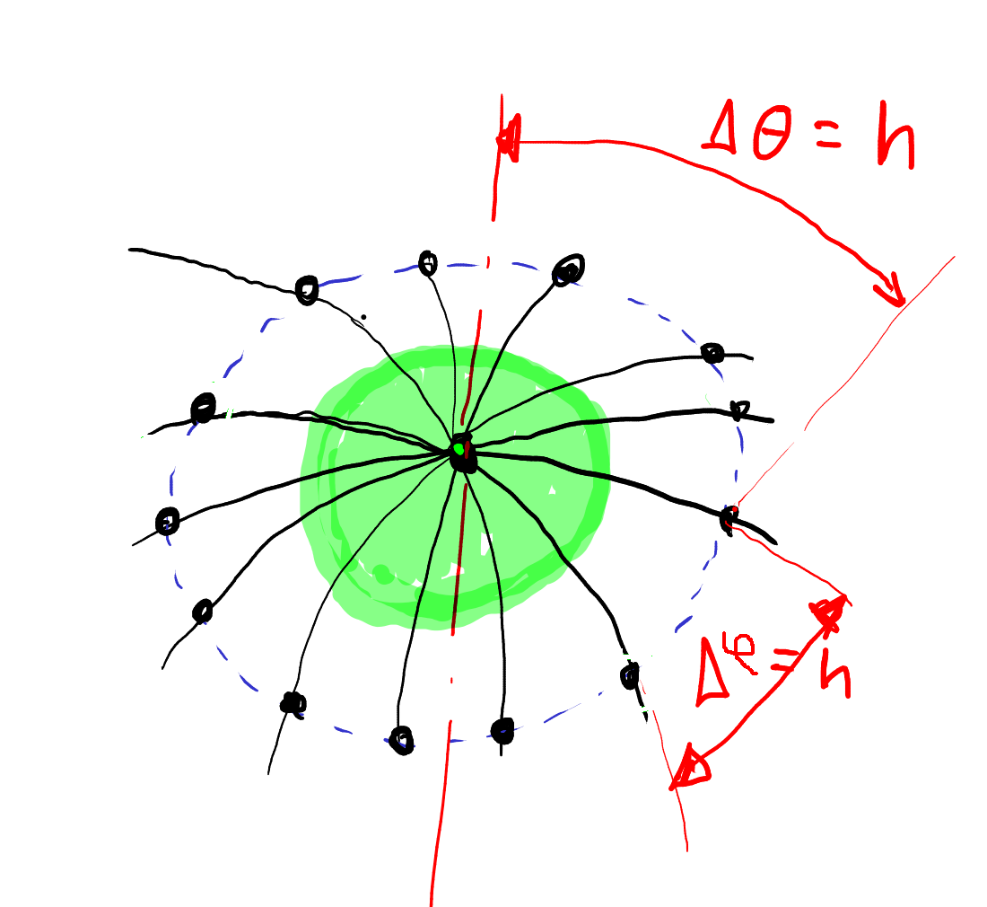
We will proceed to derive a discretization for the north pole. The discretization for the south pole can be derived in an analogous manner. Let us consider a control area of the size of the northern polar cell (green in the figure), which spans $\tilde \theta \in [0,h/2]$, $\varphi \in [0, 2\pi]$.

To avoid the singularity at the pole, we will now consider an integral form of (23), which we obtain by integrating the equation over the polar cell,

We can show that the first integral in the right-hand side of (24) vanishes using the fundamental theorem of calculus:

Similarly, we can use the fundamental theorem of calculus to integrate the second term in the right-hand side of (24) over the colatitude:

As a next step, we make the assumption that $L(\tilde \theta,\varphi)$ is a constant in the polar cell, such that we can approximate the integral on the left-hand side with a mid-point rule,

where $L_{1,i}$ is the nodal value of $L(\tilde \theta,\varphi)$ at $\tilde \theta_j=0$ ($j=1$) for any longitude position $i$. This is an approximation of the integral that assumes that the nodal value of the mid-point corresponds to the area-average of $L(\tilde \theta,\varphi)$ in the polar cell. Recall that the first entry of the array $\texttt{area}$ contains the total area of the polar cap normalized with the area of the sphere (see Milestone 3 - Averages).

We then obtain

Now, we approximate the derivative of temperature with respect to colatitude at each discrete longitude, $\varphi_i$, with a central finite-difference approximation of second-order accuracy,

and the diffusion coefficient at $\tilde \theta=\frac{h}{2}$ with a simple average,

Finally, we approximate the integral on the right-hand side of (31) with a rectangular quadrature rule to obtain

Following a similar procedure, we obtain for the south pole

with

Semi-Discrete EBM

With the spatial discretization that we derived above, we can rewrite the PDE that describes our $2D$ EBM in spherical coordinates as an ODE for each degree of freedom $(j,i)$:

where we have gathered the temperature-dependent terms under $R_{j,i}(T)$ and the sources and sinks under $F_{j,i}$.

In equation (38), $C_{j,i}$ is the point-wise heat capacity that depends on the geography (see Milestone 2 - Heat Capacity); $L_{j,i}$ is the discrete point-wise heat transfer term computed with (19) for the interior nodes, with (35) for the north pole ($j=1$), and with (36) for the south pole ($j=\texttt{n\_latitude}$); $A$ and $B$ are the outgoing longwave radiation parameters (see Milestone 2 - Radiation Modeling); and $S_{sol, j, i} = (1 - \alpha_{j,i}) S_{j,i}$ is the point-wise time-dependent solar forcing term that depends on the point-wise insolation $S_{j,i}$ and the point-wise albedo $\alpha_{j,i}$.

We can rewrite (38) in matrix form as

where $\underline{\mathbf{ T}} \in \mathbb R^{\texttt{n\_latitude} \times \texttt{n\_longitude}}$ is a matrix that contains all point-wise values of temperature, $\underline{\mathbf{ R}}(\underline{\mathbf{ T}}) \in \mathbb R^{\texttt{n\_latitude} \times \texttt{n\_longitude}}$ is a matrix operator applied on the temperature matrix, $\underline{\mathbf{ F}}(t) \in \mathbb R^{\texttt{n\_latitude} \times \texttt{n\_longitude}}$ is the time-dependent matrix containing the sources and sinks of the method, and we use the dot operator to denote the time derivative term.