Milestone 5 - Stability and Jacobian Matrices

In this chapter, we are interested in analyzing the stability properties of our semi-discrete $2D$ EBM.

Mapping from a $2D$ Operator to a $1D$ Vector

As a first step, we will first rewrite our system of ODEs in matrix form as a system of ODEs in vector form, as that will facilitate the stability analysis of the system.

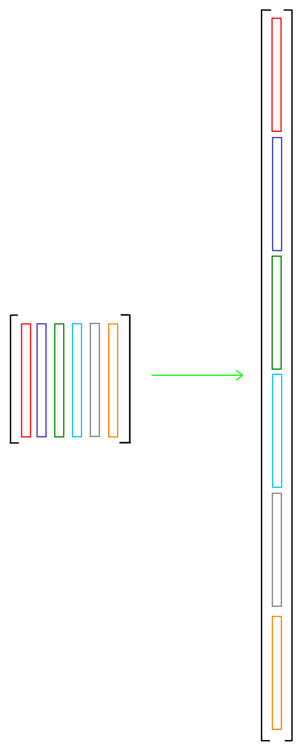
In particular, we want to concatenate the columns of our operators that are defined in matrix form (with $\texttt{n\_latitude} \times \texttt{n\_longitude}$), such that we create a one-dimensional vector with $\texttt{NDOF} = \texttt{n\_latitude} \times \texttt{n\_longitude}$ entries, where $\texttt{NDOF}$ stands for number of degrees of freedom (see figure).

Applying this mapping to our system of ODEs in matrix form, we obtain

where $\mathbf{T}, \mathbf{R}(\mathbf{T}), \mathbf{F}(t) \in \mathbb R^{\texttt{NDOF}}$.

Stability Theory for Linear Systems of Equations

As we saw in Milestone 3, the maximum allowable time-step size depends on the choice of the time discretization method for scalar ODEs. In this section, we will apply the stability theory presented in Milestone 3 to systems of ODEs that result from spatial discretizations to study the stability properties of our $2D$ EBM model.

As a first step for our analysis, we will take advantage of the linearity of the term $\mathbf{R}(\mathbf{T})$ to rewrite our system of ODEs (1) as

where $\underline{\mathbf{ A}}$ is the so-called Jacobian matrix of the system.

Note that (3) differs from the linear scalar homogeneous ODE that we analyzed in Milestone 3. As a matter of fact, (3) is nonhomogeneous and the different ODEs are coupled through matrix $\underline{\mathbf{ A}}$.

Assuming that our Jacobian matrix is invertible, we can rewrite it as

where the dense matrix $\underline{\mathbf{ V}} = [\mathbf{v}_1, \mathbf{v}_2, \ldots, \mathbf{v}_{\texttt{NDOF}}]$ contains the eigenvectors of $\underline{\mathbf{ A}}$ in its columns, and $\underline{\mathbf{ \Lambda}} = \text{diag} (\lambda_1, \lambda_2, \ldots, \lambda_{\texttt{NDOF}})$ is a diagonal matrix that contains the (possibly complex) eigenvalues of $\underline{\mathbf{ A}}$. Hence, (3) is equivalent to the system of ODEs,

where $\mathbf{Z} = \underline{\mathbf{ V}}^{-1}\mathbf{T}$ and $\pmb{\mathcal{F}}(t) \coloneqq \underline{\mathbf{ V}}^{-1} \mathbf{F}(t)$.

Note that the individual variables in (5) are decoupled due to the diagonal matrix $\underline{\mathbf{ \Lambda}}$. As a result, (5) resembles the linear scalar homogeneous ODE and the solutions have the form

where $Z^p_{i}$ is a so-called particular solution (also particular integral) for the $i^{\text{th}}$ nonhomogeneous problem that depends on $\mathcal{F}_i(t)$ and $\lambda_i$, and $a_i$ is a constant that is adjusted to match the initial condition,

In the case that

we expect that $\mathbf{Z}(t)$ converges to the particular solution $\mathbf{Z}^p(t)$ as $t \rightarrow \infty$. In such a case, we call the particular solution equilibrium solution.

We can now apply the stability theory presented in Milestone 3 to each scalar ODE of our diagonalized system (5). For systems of ODEs, we require that all values $\lambda_i \Delta t$, for $i=1, 2, \ldots, \texttt{NDOF}$, lie in the stability region of the time-integration method used.

Computing Jacobian Matrices (Numerical Jacobian)

It is possible to expand a general nonlinear operator, $\mathcal{R}(\mathbf{T})$, with a multi-dimensional Taylor series to obtain,

where the Jacobian matrix is defined as

This Taylor expansion can also be used to approximate the Jacobian matrix. For instance, one can assume that $\mathbf{T}$ differs from $\mathbf{T}_0$ only in one degree of freedom by a small quantity $\epsilon$,

where $\hat{\mathbf{K}}^j = (\hat{k}^j_1, \hat{k}^j_2, \ldots, \hat{k}^j_{\texttt{NDOF}})^T$ is a vector whose entries are defined as

Equation (10) can then be rearranged as

For general nonlinear operators, the quantity $\underline{\mathbf{ A}} \hat{\mathbf{K}}^j$ is a good approximation for the $j^{\mathrm{th}}$ column of the Jacobian matrix if $\epsilon$ is small enough. One has to be careful in choosing the size of $\epsilon$, as very small values (close to machine precision) suffer from cancelation errors, when adding up. Hence, there is some discussion in the literature available about the optimal choice of $\epsilon$. As a starting point, it is good to consider only the square root of the currently used machine precision $\epsilon_m$, i.e., $\epsilon\sim\sqrt{\epsilon_m}$ to have a good balance of accuracy and machine error cancellation issues. For a typical double precision calculation with $\epsilon_m\sim 10^{-16}$ we then have about single precision accuracy, $\epsilon\sim 10^{-8}$.

Since the right-hand-side term of our $2D$ EBM is a linear operator, (14) is exact for any $\epsilon$ and any linearization temperature $\mathbf{T}_0$, and the second and higher-order terms vanish. As a consequence, we can choose $\epsilon = 1$ and $\mathbf{T}_0 = \mathbf{0}$ to get a column of the Jacobian of our $2D$ EBM

The whole Jacobian matrix can be recovered by computing (15) $\texttt{NDOF}$ times (i.e., $\texttt{NDOF} + 1$ computations of the right-hand-side operator $\mathbf{R}(\mathbf{T})$):